Check this article, 8mm BAD probe was tested within a wind tunnel
Applications, Assembly notes. GitHub repository with 3D files
Introduction[1]
General arrangement drawing PDF. 3D printed parts can be used instead of lathe machined parts. Drawings are freely available. Check also flanged pitot section.
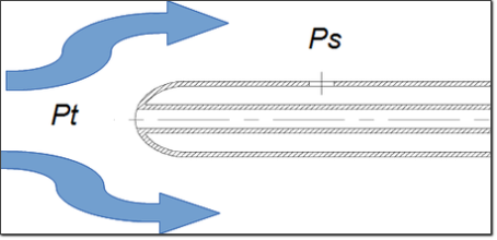
Figure 1 – Pitot Tube schematics
Widely used, the pitot tube is the backbone of air instrumentation. It’s the primary instrument for relative speed determination. Once the speed with respect to
Look at Figure 1, here you find a classic general arrangement for a pitot probe mounted on a classical nose air boom.
The pitot is assumed to be immersed in an incompressible flow. As long as we work with near to incompressible flow the Bernoulli equation yields[2][Par. 3.2], therefore in operating  [2] [Chapter 2 cover].
In this example probe, there are two pressure tap points,  stand for static pressure point and
  stands for total pressure. Imagine the probe is traveling through the air at no angle of attack at a speed of
 ![V [m/s]](http://www.basicairdata.eu/wp-content/ql-cache/quicklatex.com-1f13373d7d5ab6966edb83c9ad7e568e_l3.png "Rendered by QuickLaTeX.com") . In this condition the total pressure port sense a pressure that is[2] [ Eq 3.35] the sum of a dynamic term called impact pressure and the pressure at static tap point, whereas the flow is perpendicular to static pressure tap axis value is equal to the atmospheric pressure.
. In this condition the total pressure port sense a pressure that is[2] [ Eq 3.35] the sum of a dynamic term called impact pressure and the pressure at static tap point, whereas the flow is perpendicular to static pressure tap axis value is equal to the atmospheric pressure.
If we subtract  from
from  we get:
![\[Equation\ P.1 \qquad q_c=P_t-P_s=\frac {1} {2}\rho V^2\]](http://www.basicairdata.eu/wp-content/ql-cache/quicklatex.com-97e3c8cebd4fbe7af7bd98caf489cd90_l3.png "Rendered by QuickLaTeX.com")
This formula is the explicit relationship between relative speed and differential port pressure  .
.
The standard air conditions by ICAO is defined as follow,
The use of pitot differential pressure indication to calculate the speed with a fixed density yield to commonly defined Indicated Air Speed or IAS that is the standard speed reported by classical instruments and is not the real speed that aircraft have respect to the surrounding air.
So using the density at the standard condition into equation P.1:
![\[Equation\ P.2 \qquad IAS=\sqrt{\frac {2q_c}{\rho_{s}}}[m/s]\]](http://www.basicairdata.eu/wp-content/ql-cache/quicklatex.com-1a3ce8e2d66efd82b105e88ea8409d60_l3.png "Rendered by QuickLaTeX.com")
Sometime you can find this equation write in different ways, mainly to take care of a particular unit of measurement, as equation 4.8 in[3] that I copy here below
![\[IAS=1479.1023\sqrt{(\frac{q_c[inHg]}{29.92136})^{2/7}-1}\]](http://www.basicairdata.eu/wp-content/ql-cache/quicklatex.com-03561af5948a71ad88310c5f9f81242b_l3.png "Rendered by QuickLaTeX.com")
As a simple test of equivalence substitute the numeric values:
![\[\rho_{s}=1.225\ \frac{kg}{m^3} \qquad\]](http://www.basicairdata.eu/wp-content/ql-cache/quicklatex.com-7da8febdf6e9048175982bb330b50048_l3.png "Rendered by QuickLaTeX.com")
![\[q_c=1000\ Pa = 0.296133\ inHg\]](http://www.basicairdata.eu/wp-content/ql-cache/quicklatex.com-470b20fc46963c68a0a5661187862766_l3.png "Rendered by QuickLaTeX.com")
IAS by Equation P.1 is then 40.40 m/s = 145.46 kph = 78.5 knots;
IAS by Equation 4.8 in[3]78.5 knots;
The great advantage of using IAS is that is known that minimum take off speed is 100kph IAS no matter what are the current atmospheric pressure and temperature, the stated speed will still the same.
Compensated Air Speed or CAS is another commonly used reference speed, the basic formula is equal to IAS but a correction factor multiply the whole
![\[Equation\ P.3 \qquad CAS=cIAS\]](http://www.basicairdata.eu/wp-content/ql-cache/quicklatex.com-dce48b7e09bdab54aced6ffe2f99c4ba_l3.png "Rendered by QuickLaTeX.com")
. The correction factor c represent any deviation due to the installation of this probe on a particular kind of aircraft, anyway, also CAS does not give the current speed respect to 
![\[Equation\ P.4 \qquad TAS=CAS\sqrt{\frac{\rho_{s}}{\rho_{a}}}\]](http://www.basicairdata.eu/wp-content/ql-cache/quicklatex.com-3ec2abf8b2723d1f116aeffa957de42b_l3.png "Rendered by QuickLaTeX.com")
Let’s consider a numeric example, we calculate TAS corresponding to the same IAS in two different airfields
100kph IAS
Considering the following ambient conditions and using the standard ISA atmosphere model:
Example 1:
- Airfield alfa altitude 0 m;
- Outside temperature 20°C;
- Atmospheric pressure 100 725 Pa


Instrument reading:
- IAS = 100 kph = 27.7 m/s
- (using P4) TAS =101.2 kph / 28.1 m/s
Example 2:
- Airfield beta altitude 1000 m;
- Outside temperature 8.5°C;
- Atmospheric pressure 89 875 Pa

Instrument reading:
- IAS =100 kph
- TAS =104.8 kph / 29.1 m/s
When the actual density is lower than base density the take off rolling speed increase, so temperature rise or altitude lead to a compulsory faster take off run.
In the example the static port is located on the pitot itself, in different occasions can be located on the airplane skin, the later arrangement implicates a relevant reading error that must be compensated [4]. Sometimes the static port can be multiple, for redundancy, or annulus type, to mitigate AOA and AOS related errors.
Here I will consider some major design issues, finally, there will be a complete numeric example for
Design considerations
Pitot real behavior is close to the ideal case, however, to attain good accuracy is necessary to correct the real equation with a term that accounts for nonideal contributions.
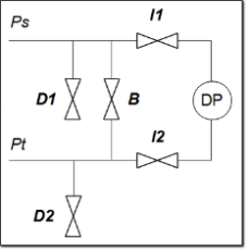
Figure 2 – Five ways manifold
Similar to the CAS formula for this purpose the multiplier C is added to the ideal equation P.1 and we get:
![\[Equation\ P.5 \qquad q=\frac{1}{2}c\rho V^2\]](http://www.basicairdata.eu/wp-content/ql-cache/quicklatex.com-1f8a9c1fc9551aa31946eb753acb789f_l3.png "Rendered by QuickLaTeX.com")
Consequently  is the difference term from ideal case,
Generally speaking, c is dependent on installation, Reynolds number, AOA and AOS[5] nevertheless many wind tunnel tests report that for some kind of pitot tubes c can be considered to be a constant at last for a well-defined speed range[5]. In
K is, therefore, dependent on the mechanical realization of the probe and the simplest method for
Typically
Pressure taps and pressure lines connection
Ideal probe exhibits a calibration coefficient that is constant over all the flight envelope so we should warrant that with different speeds the pressure tappings are performing the same way. Every pressure tap must have a sharp edge and present no burrs, the static pressure tap/taps must be drilled perpendicular at airflow at 0° AOA and AOS. The presence of round edges, burrs, and other air path modifications will lead to a speed variation of airflow and a consequently local pressure variation; also downstream blockage can lead to the same effect. Even if the pressure ports are fine
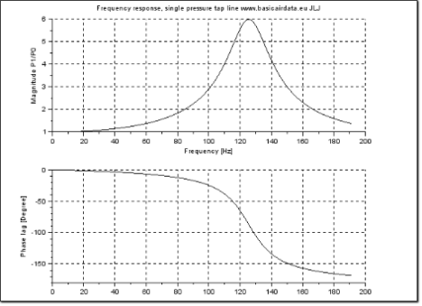
Figure 3 – Frequency response of example pressure line
It is good practice to provide a way to drain entrapped condensate from the pressure lines, it’s mandatory to entrap condensate before that reach pressure sensor, refer to the below figure as a possible arrangement. The proposed arrangement
Since the scheme is conceptual the valves in the real world can be simply replaced by plugs and pressure line interruptions. D1 and D2 represent the drain valves, locate this valves at a piezometric head below the ADC, the eventually present condensate will fill the drain lines. To ease the drain circulation consider
During pitot operation maybe some port can become clogged, sometimes it’s unavoidable to blow air from the pressure line into the probe, in this situation the priority is to don’t damage ADC sensors.
Pneumatic transmission lag
It takes some time for the pressure to propagate from the input ports to the sensors, that’s the transmission lag. Basic knowledge of this phenomenon can help to define some performance limits.
As general rule consider to maintain pressure lines as short as you can to limit pressure transmission lag[4] [pag 5][6][2] [Fig.19] and maximize dynamic response, if possible keep you pressure lines always side by side so they will be maintained at the same temperature and will have the same length; this last point ensure that the pressure is even along both the lines, no internal differential pressure buildup due to temperature differences. Pressure line material should be able to resist to condensate exposure and ensure that the lines will not deform during operations. Regarding dynamic behavior [1] [Pag 22] if the lag is extremely reduced the readings may be affected by noise due to the high bandwidth of the transmission line; that are very sensible problems, it’s not sufficient to reduce the lag but it’s also needed some degree of pressure damping.
Numeric example, data from the Pitot we will present
According to [7] [7
- Length of pressure line L= 600mmm;
- Internal line radius
 line not deformable;
 - total line volume
 ;
; - Sensor internal volume
 , depends on your sensor, probably need to be measured.
For preliminary evaluation, it can be used the Eq.3 for the asymptotic case[7] [Pag 9] that lead to a resonance frequency value of 133 Hz.
Refer to the following figure 3 to visualize the frequency response of our pressure line, this figure was calculated with
You can play around with the parameters downloading this
From the figure you can observe the resonance peak, the response of the system is unitary up to 15Hz so under this frequency the pressure transfer from the port to the sensor is ideal.
Reference [7] conclusions will clarify many interesting design aspects and since the model is validated with
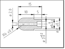
Figure 4 – Hemispherical Pitot head
When the probe is not perfectly lined with the relative wind it will perform not optimally. If the measure the AOA or AOS is unavailable the only approach is to
Design example
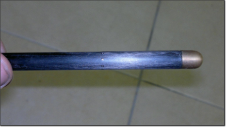
Figure 5 – Realized Pitot Head, Carbon Fiber and brass
Our design will be quite simple. First of all, we need a source for the calibration parameter and
For sake of simplicity and free online availability of documentation, our design will be based on[5]
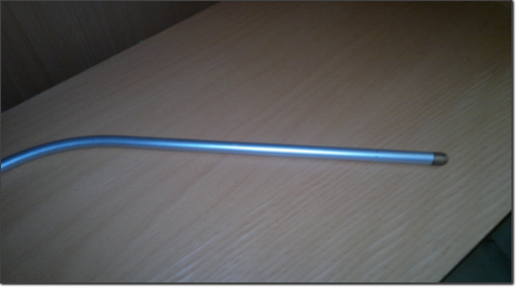
Figure 7 – Aluminum alloy detail
Because our speed formula is:
![\[Equation\ P.6 \qquad V=\sqrt{\frac{2q} {c\rho}}\]](http://www.basicairdata.eu/wp-content/ql-cache/quicklatex.com-b1ef795dba8f3fc06b9dbb91f89c5daf_l3.png "Rendered by QuickLaTeX.com")
So from[5] 
According to [5][ .
.
- 10 m/s the term
 is 191e-6
 - 55 m/s the term is 6.9e-3
In many practical cases, this term contribution can be safely neglected as it is of small magnitude.
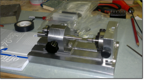
Figure 8 – DIY Dead center, drill
In [5] [1 appendix figures] you find beautiful laboratory images of the boundary layer for different
Looking for a simply realizable pitot and with a calibration factor near to 1 HNG[5][Par. 26.6 ]is chosen.
The tip of this pitot is a hemisphere, the external dimension D is 5/16” or 7.94mm, the static pressure ports are located at 4.5D from the tip and consist of one annulus of 8 holes of diameter 1.01 mm, total pressure hole is 1.84 mm[5] [Fig.1]. Measures are weird in mm as they are derived from
You find the drawing of the head
The proposed design was built and tested repeated times, obviously, you can make modifications to fit your application; i.e. find here in Figure 6 and 7 a picture of the pitot tube I realized with the same hemispheric head and aluminum alloy body.
Construction is straightforward, some problem can arise in the machining of the static ports. To allow
Now that the probe is built please go to the test section.
0 Comments