Barometric Altimeter

Page under maintenance, do you want to contribute?

Introduction

Air Data Computer project here

he Most used method for altitude measurement in airborne vehicles is by mean of static pressure readings; which is referred to as barometric altitude.

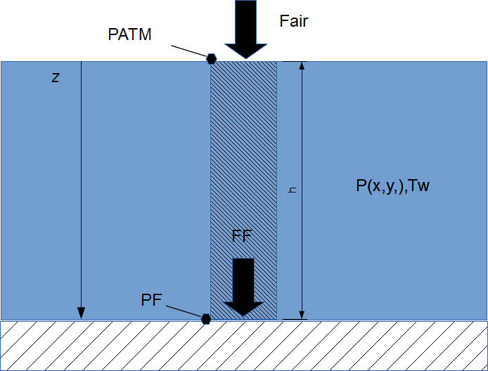
The working principle is simple and can be visualized recalling Stevin’s law for hydrostatic pressure calculation. As an introductory example, I will use the estimate of a bathtub water level. Refer to Figure 1 for a section view of a bathtub. The bathtub is filled with water at a temperature of 40 degrees Celsius while the current atmospheric pressure is 101325 Pa. Our sensor is reading the pressure on the bathtub floor that is 105000 Pa.

Water is considered still over all the tub volume, as the water pressure and temperature have a limited range of variation hence the density is deemed to be constant and equal to .

To calculate the pressure on the bathtub floor, the definition of pressure is used,

Equation 14.1, the definition of pressure:

   

Consider the force acting on the tub floor. The water layer close to the floor should withstand the weight of all the water and air that lies on top of it.
The force on the floor of is then simply equal to the force exerted by the weight of the water and the air column. The air pressure at the interface with the water is known and equal to 101325 Pa, hence we can use eq.14.1:

Regarding the water part of the column, given the gravity acceleration constant  , the water column height and taking as the column section we get: therefore

   

   

So it is practical to write
With the example data

More useful result is that the pressure at a deep is Equation 14.2:

Calculating the atmospheric pressure at a given altitude is exactly the same thing to calculating the pressure in a bathtub; it’s necessary to calculate the force exerted by the overhead air column weight.

To calculate the air density, the two prevailing models are the ISA model and the US 1962/72. For altitudes included in the troposphere, less than 11000m, they are equivalent, a vast number of altimeters use these models to convert pressure readings in altitude indications.

Below is a short list of main assumptions of the models; reference altitude is the mean sea level altitude.

a – Latitude 45°;
b – No wind or other forms of eddies;
c – Thermal gradient constant across the troposphere of 6.5 °C each 1000 meter;
d – Dry air, perfect gas
Molecular weight, from the standard air composition, is 28.9644 kg/Kmol
R=8.314462175 kJ/°K/mol;
e – Standard sea level conditions, reference conditions: ;

All the altimeters installed on aircraft have the possibility to compensate for local pressure conditions; many are capable of more sophisticated compensations for temperature and humidity deviations.
The atmosphere is by far idealized, so no local weather conditions are taken into account, all the coefficients are given to fit best at 45° latitude and standard conditions. Practically speaking, the barometric altitude reading can be amazingly off when the aircraft is flying through clouds in a hot day; tens of meters of error should not surprise us because the instrument is operating with a wrong density profile.
There are techniques to compensate for a,d and e assumptions.

Leaving to this reference the derivation of barometric formula I introduce a numeric Scilab example. In this example, two different calculation methods are employed; Initially, the barometric, or pressure altitude, is calculated using equation 4.1 from the Goodrich 4081 Air data handbook then the calculated altitude is used in the ISA/US1962/72 pressure formula. If the implementation of the direct formula is the same as the inverse formula, then the input pressure must be equal to ISA output pressure.

You can run the example and examine the calculation details (here is the Scilab barometric.sce file), and verify that results confirm the equivalence between the two methods. Just test what the Scilab output with a 105000 Pa input is.
The atmospheric model, as implemented in Scilab calculates the following data about air:

• 
• 
• 

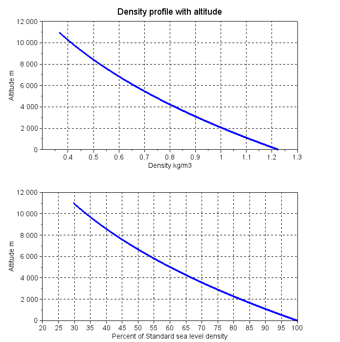
As an example calculation result, have a look at the following figure A2 that shows density vs. altitude. You can visualize the graph by setting graph=1 into the example Scilab file and executing it. The model is completed with the viscosity calculation, carried out with Sutherland’s formula. Moreover, you get the viscosity using the supplied example Scilab script.

With this data about the atmosphere, you have everything to calculate, in a practical closed form, all the performances parameters of a fixed-wing aircraft. It is so easy to have an initial evaluation of the performance of a particular airplane configuration, take off distance, climbing characteristics and in general every performance parameter inside the flight envelope.

Barometric altitude is widely used in general aviation aircraft. Use of this kind of altimeter is standard and considered reliable, and some of this reliability comes from the simplicity of the involved devices that in some cases are entirely mechanical. In terms of relative accuracy, the results are good. In the same airspace, uncompensated altimeters readings from different aircraft flying at the same altitude will be practically identical, so it’s a reliable instrument to separate flight paths of airplanes.

Unfortunately, problems arise when it’s time to land. An altimeter that follows model equations will report a wrong altitude when the plane is on the runway. This is due to the local weather conditions that lead to a different pressure at ground level.

For example, consider a runway located at 0 m MSL(mean sea level), and with 101800Pa of reported sea level pressure (by the way that is a possible value for a good autumn day in Cremona). The ISA model sets pressure to 101325 at 0 m MSL, so our altimeter is reading 101800 Pa that corresponds to -39.5 m, that, of course, is wrong.
To calculate this values launch barometricr2.sce and execute the following commands:

-->function F=isaaltitude(x)
--> F=pressure_reading-p0isa*(1-0.0065*x/T0)^(g/Rair/0.0065);
-->endfunction

-->p0isa=101325;

-->pressure_reading=101800;

-->fsolve(0,isaaltitude)
ans =
- 39.465884 

To obtain a correct measurement it’s possible to account for effective sea level pressure.
Try the following commands:

-->pressure_reading=101800;

-->p0isa=101800;

-->function F=isaaltitude(x)
--> F=pressure_reading-p0isa*(1-0.0065*x/T0)^(g/Rair/0.0065);
-->endfunction

-->fsolve(0,isaaltitude)
ans =
0. 

The last command output of 0 confirms that MSL pressure compensation is working.
If our altimeter is set up with the former method and the airfield is located at 150 m of altitude, the altimeter reading on the runway will be 150 m.
For some flight activities, such as soaring, it is convenient to know the altitude above ground level rather than the mean sea level. Pressure data is the same, but the altitude information is used to zero the altimeter indication. The sea level pressure value is available through control tower communication or from an automatic weather observation station. A typical instrument should be set up, with minor deviations, as per the Video 1

Setup should be repeated regularly during flight, or each time the pilot detects a change in weather conditions. Every variation in outside, temperature pressure and humidity will have an impact on the altimeter reading. Pilots developed some mnemonic rules to deal with this phenomenon. These rules are adequately presented in Video 2.

So if you are using a barometric altimeter to log your RC/FPV/another aircraft altitude you will need to take care of setup; pragmatically speaking, if you fly in a stable weather day and for limited time intervals and you are happy with a non-optimal degree of accuracy it is sufficient to setup your altimeter just once prior to take off. If you are willing to push to the edge of measurement state of the art, then you need to send, on a regular basis, the airfield pressure and corrected to sea level, to the flying platform.

Previously described procedures are quite standard. Considering that in many digital instruments the accuracy is constantly increased, using supplementary measurements of temperature and humidity and a more sophisticated model, the overall uncertainty is reduced. I’ll show you how our simple model can take into account temperature deviation from ISA atmosphere. Here a link to a Scilab example of altitude calculation that compensates for ISA temperature deviation. Air temperature is important because it modifies the air density profile. The following calculation examines two identical pressure readings of taken at two different temperatures and . Pressure at sea level is the standard value of 101325 Pa in both cases. Barometric altitude of P1 reading can be calculated issuing the following command:

-->exec('isatemp.sce', -1)
Input static pressure reading Pa : 100129
Pressure height 100.04 m

A check for standard thermal distribution
substituting our values results 15°C=14.35+0.65 that is exactly the temperature at sea level for ISA model. Air density is then 1.213 .
Now that the temperature profile has been checked it’s safe to assume the ISA altitude of 100 m.
Focusing on altitude:

-->exec('isatemp.sce', -1)
Input static pressure reading Pa : 100129
Pressure height 100.04 m

If altitude is the same, it’s common to say pressure altitude is the same.
Check of thermal distribution ;
substituting our values leads to 34.65°C = 34+0.65 that is 19.65°C higher than ISA expected temperature so we denote it as ISA +19.65°C or round it to ISA + 20°C
If comparison fails or measurement of pressure is not carried out in ISA conditions, some form of compensation is needed.
Air is an ideal gas here hence then:

   

   

substituting

   

Recalculate the altitude using the standard formula with our sea level temperature:

-->function F=isaaltitude(x)
--> F=pressure_reading-p0isa*(1-0.0065*x/T0)^(g/Rair/0.0065);
-->endfunction

-->T0=307.15;

-->pressure_reading=100129;

-->p0isa=101325;

-->fsolve(100,isaaltitude)
ans =
106.6349 

So the pressure does indicate a pressure altitude of 100 m identical to pressure altitude from )and compensation for the different temperatures at sea level reveals that the second reading  has been taken at 106.6 m MSL. To avoid notation confusion, the second altitude is sometimes denoted as geometric altitude.

Between the uncompensated reading and the compensated one there is a difference of 6.6 m that corresponds to a relative error of 6,2%.

Some different calculation methods have been considered, possible error sources have been introduced and basic numerical routines have been provided. The Scilab function fsolve has been used to shorten the solution but it is not usable directly on microcontrollers. For detail on implementation see altimeter implementation.

Our analysis emphasized the need for weather and altitude data at the airfield for an accurate altimeter operation.

A clarification must be made.
The barometer altimeter measures the geopotential altitude, our objective is instead to measure the geometric altitude. The two values are strictly correlated. Denoted as Geometric altitude, as geopotential altitude and as the local radius of earth hence, according to Warren F.PHILLIPS, 2009, Mechanics of Flight Second edition, Chap 1.2,

   

and

   

Of course for low altitudes the values are numerically very close and many people neglect this conversion.