[Check also alternative sensor TE-MS4525DO]
Software and basic procedures for pitot operation.
Here you can download the Arduino sketch firmware for your 8mm hemispherical head pitot circuit.
Depending on the specific application, to manage available computation power and communication bandwidth, it’s often needed to trade off on requirements.
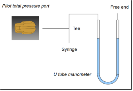
Figure 1: Tubing connection for total pressure testing
Broadly speaking our sensor board should:
- Insulate the sensor/sensor board from other electronic parts;
- Do some analog signal conditioning;
- Read signals from sensor;
- Use basic sensor calibration data;
- Run a digital filter on data;
- Add timestamp to data and manage communications;
The proposed circuit provides the mains components of a full working measure system but galvanic insulation is not implemented.
Anyway if insulation is an issue you can connect Arduino 2009 board via Xbee shield and use a separate power source/battery. To do so it is not necessary to change the sketch code, only plug in the Xbee shield; you can also choice to modify the circuit to include galvanic decouplers, for example using optocouplers IC. Decoupling is essential when is necessary to warrant the survivability to severe failure, in a harsh environment scenarios or under extreme operational safety requirements.
Analog signal treatment is not used, every related problem is left to the pressure sensor itself, sensor digital compensated output is used.
The sketch compensates for sensor zero offset, for higher accuracy it is necessary to verify the input/output characteristic for a greater number of test points. If the reading of the sensor must be interpretated with a lookup table I advise to do this operation on a higher level controller board. Also the calculation of the true air speed should be delegated to an upper level board, the main motivation is that our Arduino board don’t measure outside air temperature neither atmospheric pressure so we cannot calculate actual air density and therefore it is not possible to calculate TAS.
A useful feature is the capability to fix in a separate manner the report rate value and the sample rate value. Refer to sketch, with shown mechanism you can relief transmission line and do at the same time signal oversampling and filtering. In particular the sketch will send the data through a moving average digital filter, macroscopic effect on data consist in data smoothing.
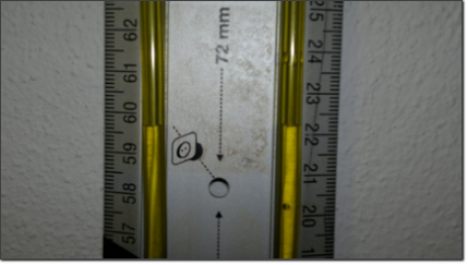
Figure 2: DIY U tube Water columns at the same height, 0 mm differential pressure
Every sample is paired with a timestamp, this value is an offset time calculated since the program start to run. The counter is a long unsigned integer and store the offset time in milliseconds, so when the count exceeds  counter will restart; that’s will happen approx after 49,71 days of running time.
Total pressure port test
Let’s proceed to check our sensor total pressure port, leaking in pressure lines and sensor problems can be in such a way detected. The easy way is to compare your reading with the measurements from a calibrated digital precision sensor(detailed procedure here), in the case this tool is unavailable we can test our pitot using a DIY vertical U-tube manometer feed by a syringe. The U-tube manometer is really easy to build, inexpensive and of course a lot theatrical, of course you can also bought one. Refer here for a figure, the pressure difference between the two tube ends is equals to  , where
  represents the difference in height of the two water columns or head.
In this example I present a procedure to test the pressure port, this procedure is really similar to a sensor calibration but it is intended here only to provide a method to detect major failures; it’s a simple procedure to use from time to time to evaluate pitot status, it’s quite common to have some leak on pressure lines or sensor drifting.
So we need to connect the pitot as show in the Figure 1.
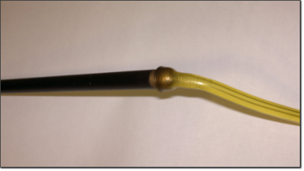
Figure 3: Pitot head ready for measurement, tube fitted
You can make your own U-tube manometer with some rigid tubing, Figure 2 shows my water filled DIY U tube zeroed and ready for port test.
The connection with the pitot head must be airtight, in the picture 3 my arrangement, I pushed the tubing over the pitot head.
To increase the total port pressure reading simply press the syringe plunger, be aware that if you push water into you sensor port you can damage your sensor.
Let’s pretend measured is 35.6e-3 m and the room temperature is 21.1°C, as reported in this spreadsheet. From the temperature you can calculate the density, there are online water density/properties calculators but for best performance refer to international authorities as NIST or BIMP methods/tables.
Here is the calculation:
![\[Pressure=997.95 \frac{kg}{m^3} \cdot 9.81 \frac{m}{s^2} \cdot (35.6e-3)\ m = 348,52\ Pa\]](https://www.basicairdata.eu/wp-content/ql-cache/quicklatex.com-06995fbe64cbc9376dceb2c26712752c_l3.png "Rendered by QuickLaTeX.com")
Referring to the spreadsheet you can notice that the example pitot is working fine, we have a matching IAS indication from Pitot board and from U-tube. To increase accuracy, for example for calibration purposes, you can use an inclined tube manometer. Measuring with U tube manometers can be really tricky, an electronic sensor setup is extremely comfortable.
Zeroing the sensor
Now that the circuit is wired it’s time to connect your Arduino board to your PC and load the sketch, at this point you should have the situation pictured here below. Note that the total pressure line of the Pitot should be connected to the pressure port named as one on the datasheet, refer to Figure 1, the other sensor port should be connected to static port on Pitot.
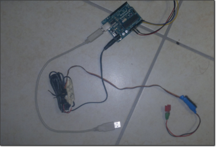
Figure 4: DIY System wired and ready to be connected to PC, BEC coonection must be removed prior to USB connection. Use BEC only is you need operate without power supply and you provide wireless or other mean of commununication interface.
Upload the Arduino sketch to board and launch the serial monitor, set the baud rate of the monitor to 57600.
Now on the screen you should see a text string composed by numbers separated by a semicolon.
The data output follow this scheme: “timebase ms; Reading counts; Raw reading Pa; Offset compensated reading Pa; Digital filtered reading Pa; IAS m/s”.
Leave your sensor at rest and collect data for twenty seconds. Untick the autoscroll box into the serial monitor, select all the data with the mouse and press Ctrl+C (windows copy) open a notepad and paste the data with Ctrll+V (windows paste) and save everything to a file. Now you have the data into a spreadsheet, refer to the example spreadsheet here. You can calculate really fast the mean and the variance of the data series.
Once you have prepared your data entry format, maybe something similar to example spreadsheet, it’s straight forward to copy and paste new data to analyze. On some systems the decimal separator is a comma, if it is the case you can substitute all the points with commas directly inside the notepad with the find and replace command rather than change your system settings. Let’s have a look to the example data, the searched value is the mean of the raw pressure, so 4,42 Pa. Check also the deviation, if you get a value that is is too high with respect to sensor expected deviation maybe you have a damaged sensor. Anyway read the average raw pressure value and use it as the offset variable value in the sketch, doing so the software will subtract this value to every sample; once done upload again the code to the board, collect again the serial outpu and update your excel file. Please find my second excel file here.This time the average of compensated measurements should be near zero, indicated airspeed should be practically zero, if not a inspection of whole system is needed. Offset compensation will be really accurate because the sensor pressure difference applied to the sensor is precisely zero.
Some details to check prior to the use of Pitot
Since I used the data from my 8mm probe the calibration factor c value was set to 0.9965790, before you operate your pitot you need to follow the test and calibration procedure to get you own pitot c. Note that into the code is implemented a digital moving average filter, it works with the current sample value and two other memorized values. It’s a really scarce low pass filter anyway it’s a good smoother in the time domain and have been included for the former feature. To achieve a good low pass behavior you need to increase the stored samples to 60 or more or use a more advanced filter.
Considerating all the uncerainty terms It’s honest to to say that IAS measuremt should have a deviation of 0.2m/s hence we can write IAS(0.6)m/s with 99.7% confidence level.
To validate the uncertainty model an experimental campain is formally needed, the required calibration effort is usually beyond DIY scope.
If any problem arise, or you need some help, fell free to contact the author directly on the blog.