The placement of the Pitot probe is a rather neglected topic which, by its nature, doesn’t have a closed form solution. This article examines this problem and provides an estimation of the resulting static error.
 Airspeed probes and altimeters rely on the measurement of static pressure. From the end-user standpoint, problems may arise when the unit is installed on the airframe: even the most accurate Pitot probe can have installation-related issues. These are commonly called “position errors” and depend on the position and orientation at which the probe is installed and on the airframe-specific aerodynamics. The probe has two pressure ports, one for sampling the impact or total pressure and another for the static pressure. Total pressure is commonly less sensitive to the installation position; we will focus on the static pressure.
Static pressure is the pressure component normal to the streamlines. In a non-compressible, inviscid flow scenario, valid for airspeeds V under  or 102 m/s, the Bernoulli equation along two points on a streamline can be written as
  .
.
Consider two points with the same piezometric height,  . The previous equation states that if the velocity of the fluid changes then the static pressure changes as well.
Any obje ct modifies the flow field in which it is immerged, so any measurement carried out inside the modified flow field will lead to a wrong indication of free stream static pressure. Precise evaluation of the pressure field, aerodynamic interferences and the measurement errors in a particular flight condition requires CFD simulation, wind tunnel runs or in-flight testing. A different approach to position error evaluation is to use system identification techniques on flight data. The strong point of the latter approach is that one can develop a fully automated procedure to evaluate position error,through post-processing of the flight data.
Let’s assume that we are content, from an accuracy standpoint, with using data from 3 rd party experiments.
As the topic is extensive, we focus on the nose-mounted probe case. Sometimes this problem is underestimated, while it really is not trivial. The generalized mounting layout is depicted on the picture at the top of the page.

Figure 1: Top Simple body of revolution meshed for CFD, JLJ
There are two variations of the problem. In the first, the static and total pressure ports are both located on the Pitot probe, in front of the nosecone. In the second, the static port is located on the fuselage.
Let’s examine the first case. The airplane motion causes a disturbance in the surrounding air, which also propagates in front of the airplane body. When the incoming air hits the nosecone, it is forced to slow down. Upstream, this is perceived as a blockage and causes a modification in the velocity field. To visualize this effect, have a look in the following CFD simulation of a simple body of revolution, inserted in an airstream at zero angle of attack, zero sideslip and a velocity V of 22 m/s.
Inspecting the Figure 1, it is apparent that the velocity field is modified ahead of the body, so even in the case of nose mounted Pitots we must expect a certain position error.
Refer[1] to naca-tn-1496 paper on Pitot static tube extending forward from the nose of fuselage.
According to figure 4 in page 17, the static pressure error decreases with the distance  , at which the static port is placed in front of the nosecone. Denoting
  as the fuselage diameter, the error curve is plotted as a function of x/D. The error is normalized with respect to the impact pressure
  . For example the elliptical nose fuselage with
  we expect an error of 4% of . In the same scenario, the circular nose fuselage body reach almost 10% error.
Judging by this plot, we observe that a streamlined body introduces a smaller error than a blunt body.
Since typically a fuselage geometry does not exactly match one of the shapes examined in that paper, it is obvious that results cannot be, strictly speaking, directly used in our applications, but an “upper bound” approach can be applied to attain a robust estimation of the pitot position error.
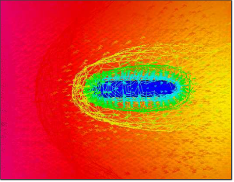
Figure 2: Bottom Iso average velocity surfaces
Let’s assume we have an airframe with a fuselage diameter of 0.15m, with a pointy nosecone. This matches the layout of an RC glider. To eliminate the error introduced in the static port by the nosecone altering the airstream, we chose a conservative  value, so we set
  . If your fuselage doesn’t have a circular section, you can use the hydraulic diameter
  instead. can be calculated as
  where
where  is the section area and
  the section perimeter. Since we are interested only in the upper bound of the estimation, you can use also the diagonal length of your section for the calculations.
In our design, the exact static error value is unknown, but it is reasonable to expect a value in the order of 5%. This is quite high and unacceptable, if you have paid for an accurate Pitot probe.
If you want to further reduce that error, the most direct method is to perform a test-flight to characterize the probe.
Another approach would be to seek an alternative installation position, such as the leading edge of the main wing. Of course, if you haven’t constraints on the overall dimensions, you can also design a longer pitot tube.