General considerations about air data instruments sensors calibration and test.
Secondary test and calibration

Figure 1: Ideal linear sensor input-output characteristic

Figure 2a : Variation of slope
Air data intruments are composed by two main subsystems, the primary that is in contact with the air stream and the secondary that represents everything else.
The secondary includes sensors, electronic interfaces and software. On a regular basis is necessary to test secondary components.
Within this document a general model for linearized sensors is examined. After a general introduction, a numeric example will be introduced. Instrument-specific calibration and test procedures, can be found on the instrument test section of the site, where available.
A sensor responds to a physical stimuli and transmits a corresponding electrical signal.
For a wide range of sensors, the relationship between input ![]() and output
and output ![]() can be approximated as linear. There are cases, however, where the relation cannot be linearized [1][2].
can be approximated as linear. There are cases, however, where the relation cannot be linearized [1][2].
The linearized sensor input-output characteristic is assumed to be a straight-line and towards that goal, the purpose of the calibration procedure is to find the straight-line that fits best the real sensor characteristic. Digital sensors can be modelled in the same manner of the analog ones. The better the resolution (in bits) of the sensor output, better model accuracy is achieved.
Defining the sensor sensitivity or slope ![]() , the offset
, the offset ![]() and
and ![]() as a random, normally distributed error variable
as a random, normally distributed error variable ![]() , the linear input-output measurement model is:
, the linear input-output measurement model is:
![]()
Refer to Figure 1-3 for a graphical representation.

Figure 3 : Sensor deviation from linearized characteristic Linearized characteristic in black and real sensor characteristic in blue.

Figure 2b: Variation of offset
The last equation explicitly accounts for the time ![]() and temperature
and temperature ![]() impact on the output. Any other negligible or uncompensated for deviation sources are formally represented by
impact on the output. Any other negligible or uncompensated for deviation sources are formally represented by ![]() . For example, in the case of a ratio-metric sensor,
. For example, in the case of a ratio-metric sensor, ![]() can the power voltage value. In general
can the power voltage value. In general ![]() should account for every environmental factor such as vibrations, humidity and acoustic noise level.
should account for every environmental factor such as vibrations, humidity and acoustic noise level.
Sensor datasheets are commonly available on the internet and publish the upper-bound of the main error sources. ![]() can be incorporated in Eq. ILS.1 with a corresponding increase in the
can be incorporated in Eq. ILS.1 with a corresponding increase in the ![]() value of
value of ![]() error variable.
error variable.
![]()
The slope and offset values are time dependent. The variation with time of this parameters have two different time scales. The long scale variation is reported on data-sheets as “long term drift”, “aging” or with similar terms. That accounts for the fact that even a stored sensor is subject to aging and consequently the input-output relationship is time dependent.
For calibration and test purposes, aging related effects can be neglected. If a reliable sensor is required then the calibration of the sensor itself should be periodically retested.
Refer to Figure 2 to visualize the impact of slope and offset variation.
The following equation will be used during linear sensor calibration.
![]()
Generally, ![]() and
and ![]() are affected by two main thermal related issues, the initial warm up of the sensor and the operating environmental temperature.
are affected by two main thermal related issues, the initial warm up of the sensor and the operating environmental temperature.
![]() drift is reported in data-sheets as “offset thermal drift” or with similar terms under the thermal characteristics section. Τhe indicated drift is the total variation inside the sensor operating temperature range. The drift of the offset value after an initial power up period is called “power up offset drift”, “warm up thermal shift” or with similar terms.
drift is reported in data-sheets as “offset thermal drift” or with similar terms under the thermal characteristics section. Τhe indicated drift is the total variation inside the sensor operating temperature range. The drift of the offset value after an initial power up period is called “power up offset drift”, “warm up thermal shift” or with similar terms.
We define ![]() as the output span or range and
as the output span or range and ![]() as the input span or range, hence:
as the input span or range, hence:
![]()
It is uncommon to find in data-sheets explicit descriptions on slope/sensitivity variation with temperature. Instead, it is quite common to have indications about input and output span deviations; usually in the thermal effects section.
Another useful piece of data reported in data-sheets is the “linearity error”. The general concept is that linearity error accounts for the differences between the sensors measurements and a best fit straight-line.
To operate in a static or quasistatic condition, it is necessary to check the response time of the sensor. Generally this value is reported as the time to reach a certain percent of the true output value.
To be sure you are operating at low frequencies check that your sample time is at least six times the time required by the sensor to reach 68% of output value. For the majority of sensors this will be an overly conservative value
Let’s introduce an example on a real sensor.
Preliminary estimation of sensor uncertainty
A reliable, digital, compensated and non ratiometric sensor is available from Sensortechnics, with part number HCLA12X5B. The datasheet can be found online at this link.
This sensor measures differential pressure input and represents it with a hexadecimal value. Its nominal range is from -1250Pa to 1250Pa.
Let’s estimate the out-of-the-box expected uncertainty of measurement. Of course, that is the uncertainty we attain if we use the nominal values reported into the datasheet or implicitly assume a linear model for our sensor. In this preliminary analysis, the statistical distribution of error will not be taken into account; instead, a worst case approach is used. On those assumptions, the concept of uncertainty is almost identical to the error.
The wiring scheme of the HCLA sensor and some basic firmware can be freely downloaded from here.

Figure 5: Plot of collected data and zoom view of the same data
We assume that all uncertainty contributions are statistically independent with respect to the others. Refer to page four of datasheet to retrieve all the sensor performance-related numerical data.
Datasheet reports an expected zero pressure offset between ![]() or
or ![]() and
and ![]() or
or ![]() , with a central value of
, with a central value of ![]() or
or ![]() .
.
The nominal output span is (-12,5mBar,12,5mBar) or ![]()
![]()
For the sake of simplicity, from now on we will use the decimal notation.
In the given output span, every decimal count corresponds to a ![]() Bar change or 0,0953 Pa.
Bar change or 0,0953 Pa.
Let’s examine the offset related uncertainty terms.
The initial offset value can have a variation range of ±655 counts over a nominal full span variation of 26214 count, otherwise stated 2.5% full scale span. At the same time “Thermal effects (-25 to 85°C)” can cause a change to the offset of 1%FSS. To further reduce the performance, the term of “Offset warm-up shift” must be considered. The maximum rated value for this parameter is 33 counts or 0.13%.FSS.
In the worst case scenario, without warm up offset correction, the sensor will have an uncertainty of 3.83 %FSS. For our sensor this corresponds to 96 Pa. Using IAS definition this value leads to a reading of about 12.5 m/s or 45 km/h. So if the sensor is used with a Pitot probe, we can expect an erratic speed indication even when the Pitot is at rest on the table.
Now that the offset is evaluated, we must also add the uncertainty caused by span variations.
Page four of the datasheet reports that full scale span is in the interval ![]() or
or ![]() and the center value is
and the center value is ![]() or
or ![]() .
.
Using equation ILS.4
![]()
![]()
![]()
In this case the uncertainty value is proportional to the magnitude of the measured ![]() pressure count.
pressure count.
![]()
Or in a relative form
![]()
The uncertainty due to hysteresis and non-linearity ![]() is considered to have a maximum value of 0.25% FSS. This should be further expanded upon, but I choose not to make this discussion for now.
is considered to have a maximum value of 0.25% FSS. This should be further expanded upon, but I choose not to make this discussion for now.
Until now we have a total uncertainty of ![]()
If we consider the bare value of 6.68%FSS, the sensor seems to have poor performance, but it is not the case. First, we should note that this uncertainty estimation corresponds to a full swing of the output. Even if this is formally correct, it is unrealistic to use that value as a single pressure measurement uncertainty indication. Typically, we can get a much better measurement because we usually operate in the central region of the output range.
Is now quite clear, that the use of the sensor which is treated as linear, using nominal values, leads to an unacceptable level of uncertainty. So what we need to do in order to get a better measurement?
A viable procedure is to reduce the offset and sensitivity uncertainty term By removing those terms, we get ![]() .
.
To achieve a result of this grade, it is necessary to compare our sensor readings against a reference manometer. To compensate for temperature-related deviation of the bias over the operating range requires collecting a hefty amount of experimental data. Details on the procedure will be presented on the following sections.
Statistical behavior of the sensor
Usually datasheets do not report statistical information. To reach top notch measurement levels it is necessary to collect statistical data for the sensor. This may seem a bit cumbersome but it can be done with a reasonable amount of effort.
Information about statistical distribution allows us to have a better indication on the most probable measurement value. There are a few statistical distributions that can be employed to model sensor data. In this text, our approach is to use experimental data to construct the probability density function of our sensor.
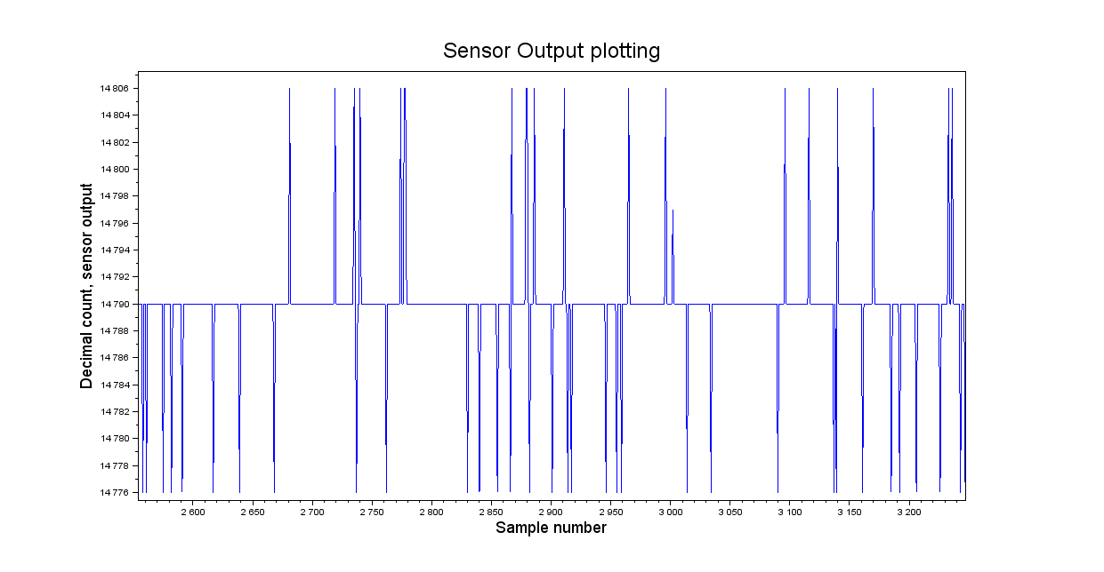
In this link you can find 16870 pressure samples collected from a HCLA12X5B pressure sensor at a sample frequency of 10Hz. The two pressure ports have been left unconnected to have a zero reading. As room temperature is constant and the input is fixed to zero we expect to have a data set without any trend. By inspection of the plot of the sample data in Figure 5: it seems this is a correct assumption.
With the current level of approximation, a reasonable simplification is to consider the samples as uniformly distributed.

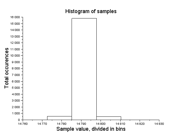
Figure 6: Histogram of experimental data

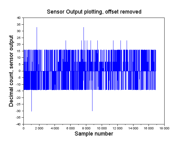
Figure 7a: Plot of z, samples without offset

Figure 7b: Plot of z, samples without offset
This distribution model assumes that every possible value within the full measurement span has the same probability of appearing.
That assumption allows us to write
![]()
![]()
![]()
To verify that this value is representative, it is necessary to take different data series at different pressures. For this sensor, the experimental deviation (uniform discrete distribution) at full scale was calculated as ![]() , so the sensor seems to perform better at higher pressures. In uncertainty propagation analysis, we consider the worst case. We will examine the uncertainty of the measurement offset as an example of all the other quantities, for the sake of keeping the introductory procedure simple.
, so the sensor seems to perform better at higher pressures. In uncertainty propagation analysis, we consider the worst case. We will examine the uncertainty of the measurement offset as an example of all the other quantities, for the sake of keeping the introductory procedure simple.
Two data series are not enough to consider the analysis completed. A more accurate analysis will require logging many more sensor responses at different pressures. The more data series you collect, the better uncertainty figure of the sensor you can achieve. Also recall that uncertainty is tightly correlated with operating temperature. To minimize the number of data samples collected is necessary to previously evaluate and define the operating conditions of your differential pressure sensor. For example, if you plan to take a huge number of pressure measurements around 1000 Pa, then it is wiser to collect experimental calibration data around this pressure rather than collecting data all over the full pressure span.
By executing this Scilab script, the measurements histogram ILS.6 is plotted.
Additionally, along with other results, the number of occurrences per each value is displayed:
Decimal output / #counts or frequency
14790. 15516.
14776. 536.
14797. 294.
14806. 501.
14760. 2.
14823. 2.
14813. 9.
14783. 10.
14790. 0.9197392
14776. 0.0317724
14797. 0.0174274
14806. 0.0296977
14760. 0.0001186
14823. 0.0001186
14813. 0.0005335
14783. 0.0005928
Table 1 Frequency counts
As you can observe from the histogram, the data probability distribution does not have a Gaussian <link> bell shape. The data have a strong mode; in fact 92% of samples are exactly 14790 and the distribution is symmetric. The data buckets that have been used for the histogram plot do make the difference in visual inspection. To verify this, visualize the same data with fifteen classes; change the supplied script line 17,or issue a new command, from “histplot(5,y,normalization=%f)” to histplot(15,y,normalization=%f). This way you will see the same data divided in 15 classes. With 15 classes for the histogram you get multiple void bars and the histogram seems asymmetric. To avoid such a misleading plots use classes with, pragmatically speaking, at least 10 samples.
It’s reasonable to use 14790 as the most representative value, bet let’s check the mean value ![]() anyway. Let’s denote
anyway. Let’s denote ![]() as the ith sampled value and
as the ith sampled value and ![]() as the probability function.
as the probability function.
![Rendered by QuickLaTeX.com \[\mu_s=\sum_{i=1}^{14790} y_i p(i)\]](https://basicairdata.eu/wp-content/ql-cache/quicklatex.com-86025ba735fd11d624b9119b6c2d288f_l3.png)
The mean value is 14790,16. Having decimal parts in values leads to treating all data as float numbers. However, sometimes it can be also acceptable to round to the nearest integer. This value seems good as is inside the manufacturer-specified range for offset of ![]() .
.
The standard deviation of the samples can be calculated as:
![Rendered by QuickLaTeX.com \[s=\sum_{i=1}^{14790}{ (y_i-\mu_s)^2p(i)}\]](https://basicairdata.eu/wp-content/ql-cache/quicklatex.com-d1b55cae5c95eace8c733f133d106575_l3.png)
that yields to a value of 3,89 Pa.
The minimum value of ![]() is -30,1 Pa and maximum 32,8 Pa. Sure, the dataset has some outliers in it, but recalling that 92% of the measurements where equal to 14790 and the samples within one standard deviation
is -30,1 Pa and maximum 32,8 Pa. Sure, the dataset has some outliers in it, but recalling that 92% of the measurements where equal to 14790 and the samples within one standard deviation ![]() represent 95% of the total, I do not apply any further refinements to the model.
represent 95% of the total, I do not apply any further refinements to the model.
Setting offset value for pressure measurements
Returning now to our former problem of offset compensation it makes sense to use 14790,16 as the ![]() offset value, hence the measurement without offset
offset value, hence the measurement without offset ![]() is written as:
is written as:
![]()
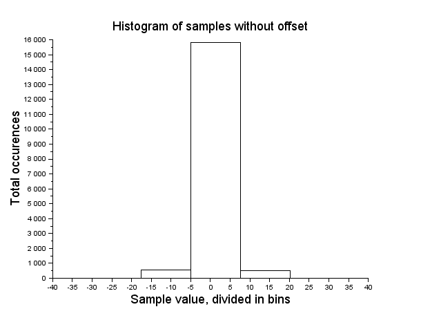
![]() has the same statistical pdf as
has the same statistical pdf as ![]() .
.
Since the offset is compensated, the mean of ![]() should be very close to zero. In our case it is pretty close, with a 5.732e-13 value. If the model is acceptable,
should be very close to zero. In our case it is pretty close, with a 5.732e-13 value. If the model is acceptable, ![]() contains all the dynamics, so the expected variance of
contains all the dynamics, so the expected variance of ![]() is identical to the variance of
is identical to the variance of ![]() . A fast verification with the Scilab script leads to assertion that the two values are identical.
. A fast verification with the Scilab script leads to assertion that the two values are identical.
With this systematic approach we finally get a really trustworthy offset value. The deviation ![]() of the average of all the pressure measurements gives us an indication of how much we can rely on our offset measurements. In our case
of the average of all the pressure measurements gives us an indication of how much we can rely on our offset measurements. In our case
![]()
![]()
Tackling the offset warm-up drift
The manufacturer reports the value of the offset warp-up drift. Let’s verify this with a one hour long pressure log. Prior to testing, the sensor is stored for a long period of tie, say few hours.
We will conduct two different tests, whose parameters are reported in the following table. Note that in order to identify the warm up behavior a more extended experiment is needed.
To load and compute data please refer to Scilab file “datacrunchpitot2.sce” and data files “hcla12x1hz 8 deg C looking for drift” and “hcla12x1hz 20 deg C looking for drift”.
Take a look at Figure 9. A trend line is superimposed to the raw data and the smoothed data. A moving average filter , that averages 100 samples each time, is used. The trend or regression line is calculated using the least squares criterion.
| CASE# | Instrumentation rest period before data collection | Sample rate | Room temperature average | Slope of trend line | Offset | Standard deviation of the residual |
|---|---|---|---|---|---|---|
| 1 | 4 hours | 1 Hz | 8°C | 169.55.00 | -330.43.00 | 09.00.00 |
| 2 | 4 hours | 1 Hz | 20°C | 301.35.00 | -59.53.00 | 09.08.00 |
Table 2: Test data
In case #1, after one hour, the drift span value is equal to ![]()
Instead, in case #2, we get ![]()
The expected maximum span is ![]() . Considering that only one data series is collected for each case and assuming that the linear approximation is representative of the data series, the offset warm-up drift seems to be compatible with the value stated into the data-sheet.
. Considering that only one data series is collected for each case and assuming that the linear approximation is representative of the data series, the offset warm-up drift seems to be compatible with the value stated into the data-sheet.
Measurement of the actual slope of m

Figure 9: case #2 – Plot of data with trend line and smoothed data
It is important to measure and calibrate for the slope of the output. To that end, we need to log measurements for the full output scale. Both the positive and negative ranges should be checked, but for the sake of simplicity, only the positive pressures will be considered in this text. The input-output characteristic is assumed to be a continuous line crossing zero and spanning all the way to full scale measurements. A formal approach is to collect measurements at different pressure values and then do a best line fit, but for now we will take a simpler approach.
The most important piece of hardware in this process is the reference manometer. The manometer should be calibrated prior to the sensor test. This should be done in order to determine the measurement uncertainty.
For example purposes let’s assume that our reference manometer has 6 Pa of uncertainty ![]() and the sensor under test, as previously stated, has 18 Pa of uncertainty
and the sensor under test, as previously stated, has 18 Pa of uncertainty ![]() .
.
All the measurements should be conducted in a room with stable temperarture, otherwise a variation in recorded pressure is to be expected. A variation of 0.5°C along the test have been proven to be an acceptable room temperature change. To connect a pressure source to both the reference and the sensor under test, some sort of test rig is needed, I use the arrangement shown in this link
The data processing can be carried out with “mslope.sce” Scilab file, data is stored in “hcla12x10Hz 1250 Pa” file.
From data-sheet full scale pressure ![]() is equal to 1250 Pa, full scale decimal counts
is equal to 1250 Pa, full scale decimal counts ![]() is 27852 and zero pressure offset
is 27852 and zero pressure offset ![]() is 14745
is 14745
The ideal slope is calculated as
![]()
![]()
To check the slope/gain/sensitivity value we compare the sensor output with the reference manometer reading at full scale.
| CASE# | Instrumentation rest period before data collection | Sample rate/Samples | Room temperature average | Uncertainty | Sensor Offset | Pressure reference value |
|---|---|---|---|---|---|---|
| 3 | 4 hours +1 hour of power on period | 1 Hz/15 10 Hz/150 |
20°C | Reference 6Pa.
Sensor 18 Pa |
14790 dec counts | 1250 Pa |
Table 3: Test data for slope testing
Judging from the data, the average of the sensor measurement is:
![]()
Hence:
![]()
During data collection, the reference instrument reported a constant 1250 Pa value, with uncertainty ![]() . This is rounded to 2 Pa.
. This is rounded to 2 Pa.

Figure 9: case #1 – Plot of data with trend line and smoothed data
The average of the sensor readings has an uncertainty of ![]() . This is rounded to 2 Pa.We assume that the variance of
. This is rounded to 2 Pa.We assume that the variance of ![]() measurement is the same as every other measurement.
measurement is the same as every other measurement.
Using the uncertainty propagation formula we calculate the uncertainty of the slope m:
![]()
Concluding remarks
We’ve examined the real input-output characteristic of a differential pressure sensor. The same procedure is easily applicable to a broad family of linearizable sensors.
Collecting the results of this basic example we write:
![]()
![]()
![]()
![]()
The uncertainty of ![]() is:
is:
![]()
Equivalently we can also write:
![]()
In the last form ![]() ,
, ![]() ,
, ![]() are deterministic variables.
are deterministic variables.
Please note that the stated ![]() is not to be interpreted as the total measurement uncertainty. It is necessary to add the non linearity error, to the least. To increase the reliability of the model, more calibration steps are needed.
is not to be interpreted as the total measurement uncertainty. It is necessary to add the non linearity error, to the least. To increase the reliability of the model, more calibration steps are needed.
The uncertainty related to the thermal behavior of the sensor can be accounted for using a look-up table containing ![]() ,
, ![]() and (\sigma_y\) values at different values of temperature. The sensor model remains the same but the coefficients are calculated as a function of temperature conditions from a look-up table.
and (\sigma_y\) values at different values of temperature. The sensor model remains the same but the coefficients are calculated as a function of temperature conditions from a look-up table.
The presented calibration procedure is based on two single points and, among other things, a linear approximation. Due to the simplicity of the model, it’s possible that for many input pressure values the uncertainty value is brutally overestimated.