(This article is a digression from main requirements specification topic. You find the Pitot Static calibrator requirements reference article here)
We were concerned about the performances of the valves that should be employed into the Pitot-Static calibrator. In particular we wanted to evaluate the behavior of a valve during transitions between two different pressures. As performance test we will simulate the valve behavior when it is used to regulate the pressure of a tank. That tank is the idealization of the pneumatic circuit volume from the pressure sensor to the static port. Simulation objective is to support the Pitot-Static calibrator pneumatic circuit design, in particular the selection of air volumes. The designer should be able to easily evaluate the use of different valves.
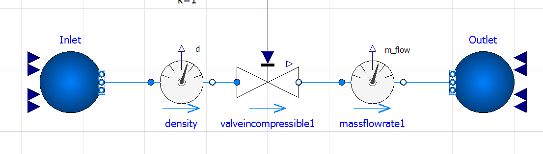
Figure 1 – Simulation setup
Valve producers provide on their data sheets a standard set of parameters to describe the valve characteristics. We will be focus here on the valve flow factor.
The flow factor correlates the flow rate to the differential pressure across a valve. There are many alternative and equivalents definitions of the valve flow factor, we will use the  factor. We define
  as the volumetric flowrate,
  is the pressure across the valve and
  is a constant dependent on the fluid type and conditions.
![\[K_v=K(\rho,p)\dot{V}\sqrt{\frac{1}{\Delta p}}\]](https://basicairdata.eu/wp-content/ql-cache/quicklatex.com-164cf6339df91c148fd878dfafb8123e_l3.png "Rendered by QuickLaTeX.com")
Find in this link the definition of from a valve producer site.
For the liquid case the given formula is:
(Eq.1) 
If the valve is tested in a laboratory setup, with water at  and with a differential pressure of 1 bar the equation is reduced to
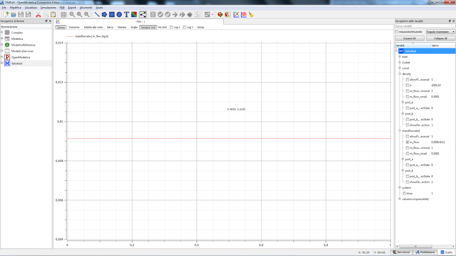
Figure 2 – Simulation results
The measured flowrate is the value. unit of measurement is that of a flow rate, a widespread used unit of measurement is  .
.
Just as reference the International Society of Automation defines the flow equations for control valves in his standard ISA-75.01.01, the correspondent European code is EN60534-2.
OpenModelica https://openmodelica.org/ has a built-in library for valves, hence I decided to simulate the regulated valve behavior using this software. At first I’ve setup a simulation to check the simulated value. You find here “valvetest.mo” file that was used for simulation; here below a figure of the simulation setup.
The valve datasheet reports  , in the simulation I’ve setup the equivalent
  . Test fluid is water at 4°C. Inlet is an ideal fluid source and outlet is an ideal fluid sink.
The valve opening can be set, for our test purposes is set to full open. All the classes used are from standard OM libraries.
Since we need the water physical properties it is necessary add to the “valvetest.mo” class header the following fluid definition:
... replaceable package Medium = Modelica.Media.Water.StandardWater constrained by Modelica.Media.Interfaces.PartialMedium ...Every component that deal with fluid must have a reference to that class. For example at the inlet fluid source we have to redeclare the Medium package:
... Inlet(redeclare package Medium = Medium, p = 200000, T = 277.15, nPorts = 1) ...After a simulation of one second we get the output shown in figure 2.
The stated mass flowrate “m_flow” is 0.00914111 kg/s, the fluid density  is 1000.02 kg/m^3. The volumetric flowrate
  .
.
The result is in accordance with the expected result that is  . Is to be note that density is not exactly 1000
  ; the density deviation requires to apply a multiplicative correction factor to equation 1:
  . Since we’re working on a robust method for a rough draft I don’t push further the research for a perfect match of the two results; it is well intended that such a topic is really interesting.
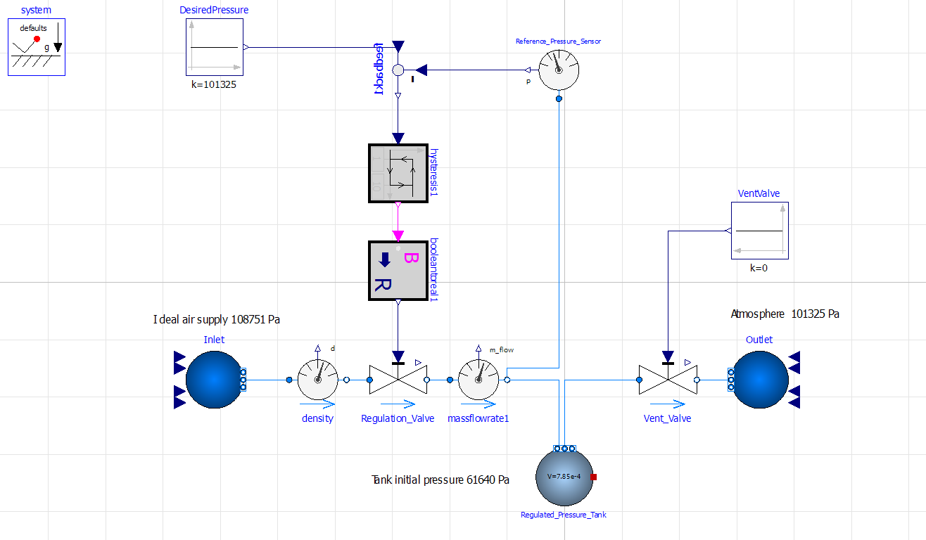
Figure 3 – Valve and primitive bang-bang regulator
Now that our valve simulation seems to work as expected let’s introduce a simple bang-bang regulator into the schematics. Refer to figure 3.
You can download here the simulation model.
The air supply is set to the maximum required pressure, the fluid sink is at atmosphere conditions. The regulated pressure tank is initialized at the minimum required pressure.
The pressure into the tank is measured by an ideal pressure sensor that feed the feedback loop. Th e desired pressure is set by a constant signal source; Pressure regulator is not fully implemented; It works only when the set point goes from a low level of pressure to a high level of pressure.
In this model the “Regulation_Valve” rise time is set to 15ms, that value comes straight from the datasheet. The regulation error is correlated with the valve dynamic characteristics, if a valve with no dynamics is used the regulation is zero.
In the supplied model the volume of the regulated pressure tank is set to a guess value of 7.85e-4  ; that is the volume of a cylindrical vessel of 100mm of diameter and height.
Pressure regulated volume idealize the internal volume of the regulated static pressure piping of the Pitot-Static regulator. Have a look to the following simulation, the pressure is regulated from an initial value of 61640Pa to 10000Pa.
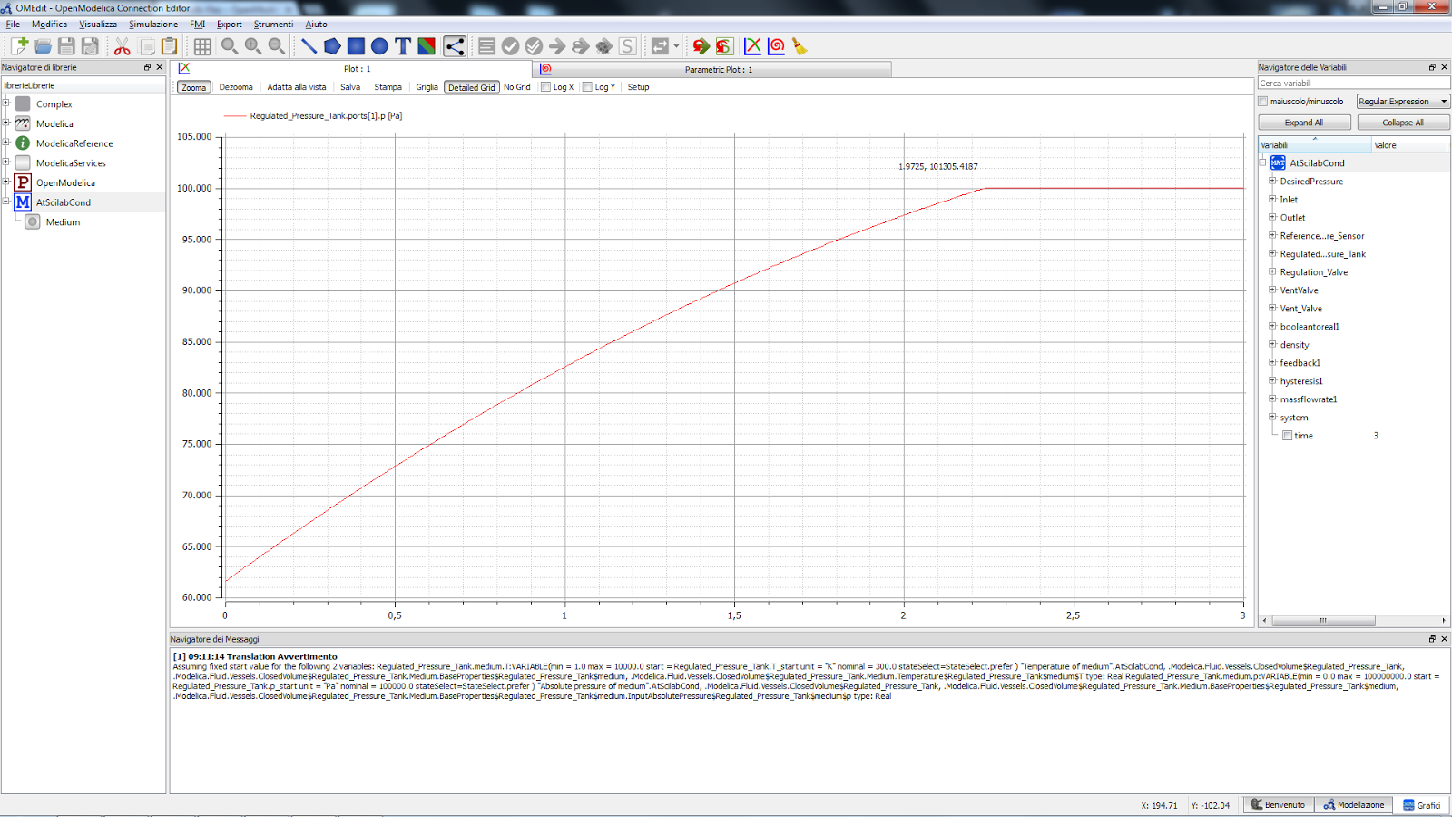
Figure 4a – Three seconds simulation
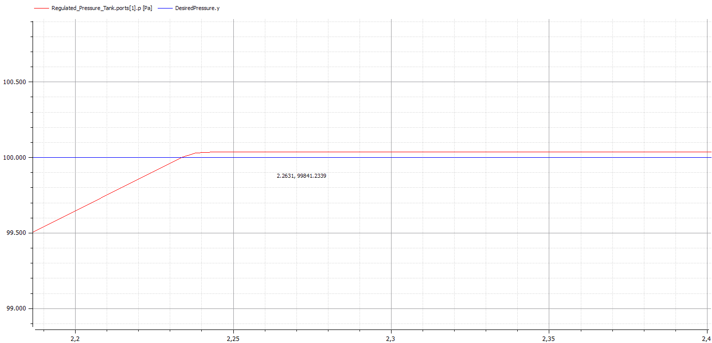
Figure 4b – Magnification
From the figures is evident that the regulated pressure doesn’t reach the desired value too well. When the pressure reach the desired value the valve starts to close, since the shut-off is not instantaneous the pressure continues to rise and leads to a pressure overshoot.
For design purposes the most important part of the graph is the pressure transient ramp, in particular is important to keep under control the maximum pressure gradient. The gradient can be limited with a higher volume tank or with a restriction orifice installed downstream the valve. The design impact can be simulated modifying the regulated pressure tank volume or lowering the value.
In figure 5 you find a plot that correlates the mass flow to the regulated pressure value, that plot provides a clear indication for the sizing of the air compressor.
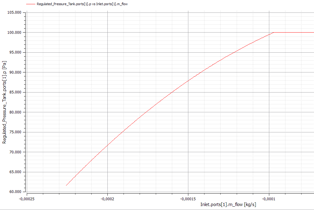
Figure 5. Flowrate VS Regulated pressure
It is possible to calculate in closed form the maximum gradient and the maximum flowrate, download here this “size.sce” script.
We will compare the Script against the simulation result, in particular the slope of the pressure transient. Using the data from simulation the slope value is calculated as the final pressure minus initial pressure divided by the elapsed time. The data of five simulation runs, with different time spans, is reported into the following table.
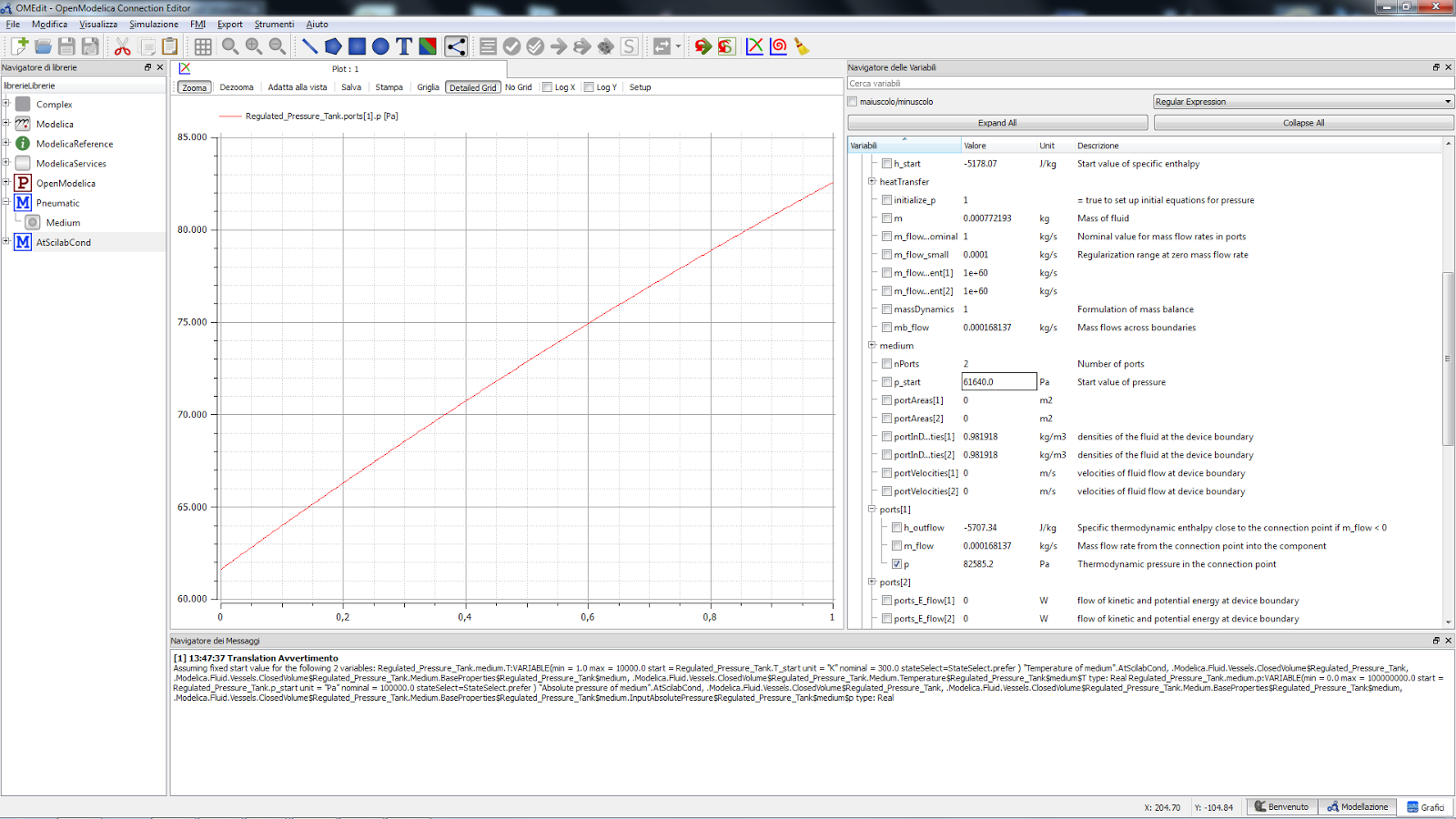
Figure 6 – The first Simulation from table 1, you can read the initial and final values from the variable browser
AtScilabConditions.mo
61640 Pa to 82585.2 Pa in 1 s
Slope 20945.2 Pa/s
61640 Pa to 64009.7 Pa in 0.1 s
Slope 23697 Pa/s
61640 Pa to 62832.5 Pa in 0.05 s
Slope 23850 Pa/s
61640 Pa to 61664 Pa in 0.001 s
Slope 24000 Pa/s
Size.sce
Max Slope
24231.6
Table 1 – Simulation VS Script numerical results
Recalling figure 5 and equation 1 we can appreciate that initially the flow through the valve is at is maximum value then it decreases, that leads to have the maximum pressure derivative for  . That fact is comforted by the convergence to the Scilab calculated value for smaller simulation intervals.
The Scilab script reports a maximum flowrate value of  , that value is in accordance with simulation value of
  .
.
(So it seems, not formally of course, safe to forward to our design team the Scilab script. We will continue with the requirements in the next article.)