Pitot Lag and Simulation
Some time ago at the airfield playing around with a pressure sensor with a sample rate of 50 Hz, I noticed an inferior unexpected performance of my carbon fiber Pitot. You know, the measuring system is quite simple, one digital pressure sensor connected to an Arduino board, two pressure lines, the static pressure port, and the total pressure port. I ended the post fly analysis with a sole sure fact. I haven’t a math model for the pneumatic transmission line. I needed such a model to calculate the relationship between the amplitude of the port pressure and the pressure at the sensor at different frequencies; synthetically I needed the transfer function. With a transfer function, it is straightforward to determinate the overall measurement system performance and even compensates for undesired transmission line behavior. Refer to the below figure 1 for the schematics of a pneumatic line.

Input pressure cannot be present at the very same time at the pressure port and the sensor port. It takes some time for the pressure wave to propagate through the transmission line.
At last, I found a text where the authors integrated the Navier-Stokes equations to achieve a closed form solution, from now on I will proceed according to reference[1] [Theoretical and experimental results for the dynamic response of pressure measuring systems].
Is very important to considerate the model assumptions, here below the list from [1] page 7
Length/Radius >> 1
Variable nominal values variations are small
Laminar flow inside the tubing
To get to a numeric example, let’s pretend we have the following, possible, parameters values
Internal radius R of line [1 ; 2 ; 3] mm
Length of pressure line L 0,6 m
Volume of the sensor Vu 50e-9 mm^3
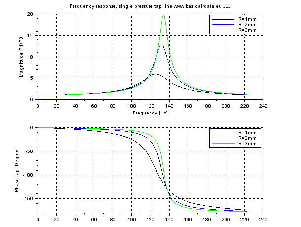
Let’s consider now three different cases from the same base design, only variable is the line inner radius R, results plotted in the decimal scaled graphic below.
You can download the scilab source here
By inspection of the figure, it’s correct to assert that if the radius increase the frequency of resonance is increased too, with a broader transmission line volume the pressure transmission and the resonance have a higher magnitude. Without correcting our sensor readings we can use only frequencies that have a gain equal to unity, so it’s clear that transmission lines can have a substantial impact on the performance, according to figure 2 we can use the frequencies safely under 15 Hz.
During the use of an instrument in non-steady conditions the frequency of pressure variation at pressure ports should be considerate. Operating with a broader bandwidth may have some drawback, the first of all is some degree of increased vulnerability with respect to unwanted pressure oscillations due to buffeting or eddies, or other sources of noise.
In figure 1 schematics the transmission line have a constant diameter, by experience, that it’s more common to have at last one variation in the line diameter, this case is well covered by papers and maybe worth a future post.
Reference [1] has a plethora of figures that illustrate different cases. Also, the conclusion section is quite clear and concise; it worth the time to read through it.
So in the end, the problems that I’ve got in the past can be explained, and some times avoided, taking into account the dynamic of the pneumatic line.
Simulation
Simulation is one of the essential tools for modern instrumentation design. Numerical simulation can be used during the early design stage as well during the final integration phase. It’s a very flexible tool and due to its intimate mathematical nature can take different forms. Even more, the same software can carry out the simulations, and do software in the loop and hardware in the loop tasks, so the development of complex systems speeds up. Simulation is also needed, for example but not only, during system identification and data validation tasks. I will show how to make a simulation of a DIY Pitot tube with Scilab, the model parameters will be set up into the
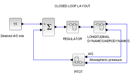
Models and simulations can be set up in different ways; I’ve chosen an Xcos block intended for continuous time simulation in the optic that usually it will be integrated into a closed-loop regulator. Refer to the following figure for a possible layout that can use our Pitot block. The scheme is quite simple as our goal is to describe pitot model usage.
At first, our concern is to have a good math representation of the physical behavior of a pitot tube, that information can be gathered from a previous analysis. At a glance, the predominant phenomenon is the pressure lines pneumatic lag. The reference shows how to calculate the response of the system at different frequencies; the used math model was validated by the authors with experimental data, so it’s safe to rely on it. Albeit the reference report precisely the relationship between input and output pressure it’s comfortable to have that information under the form of a linear low order transfer function. Since we dispose of the behavior of pitot tube in the frequency domain it’s possible to identify a transfer function that leads to this behavior, the command fdt=frep2tf(frequencies,
Identification is reasonable. You can visualize it running this file (
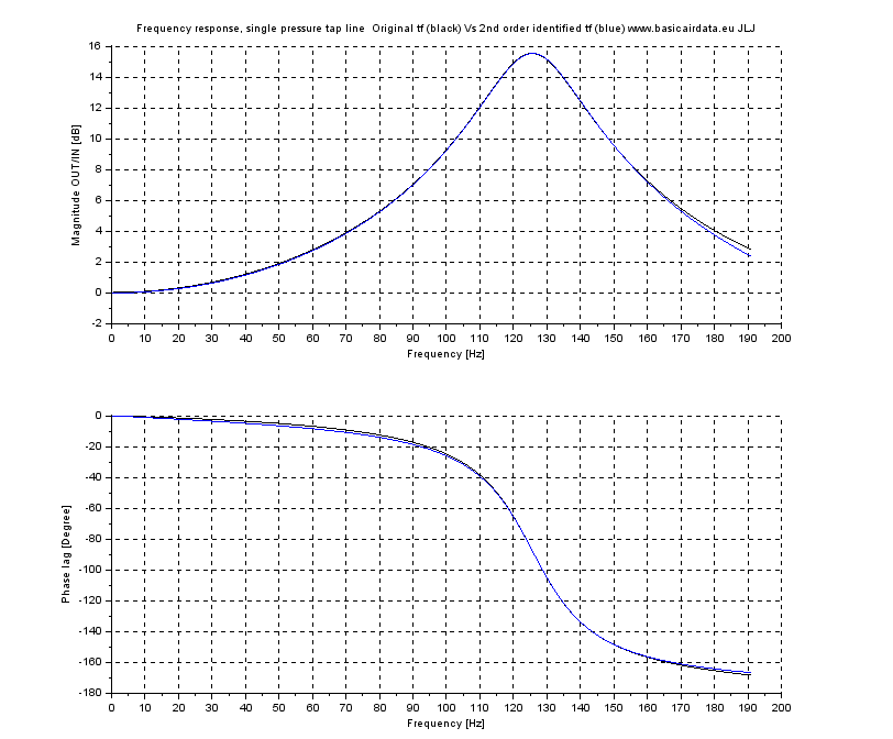
When the frequencies are under 8Hz the pressure present at the sensor is precisely the pressure at the port, as frequency increase the transmission line act as an amplifier up to the resonance frequency (in the figure PS.2 125,5 Hz). When the resonance peak effect vanishes the pneumatic line act as an attenuator, you can have a look to the transfer function issuing the command ‘q’ at the Scilab command prompt, also look at the root locus with the command
Let’s set up a simple Xcos test layout. Check the following figure for the proposed open loop test bench. For your ease download Xcos file here, parameters are those contained in
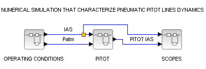
The operating conditions block generates an IAS periodic waveform, to reproduce some gusting(link) at the desired frequency, and supply the pitot-static port with the current atmospheric pressure. Scopes section collects IAS from operating conditions, real-world status, and from pitot reading, with this data the plot of Pitot error=(IASreal-IASPitot) can be visualized.
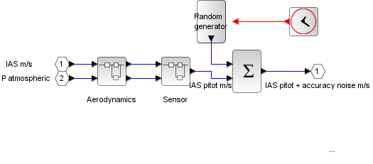
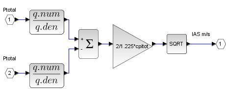
In figure PS4 you can have a look at the pitot block internals. The first block calculates the total pressure at total pressure port using as input IAS, so it passes Total pressure Pa and Atmospheric pressure Pa to the Sensor block. Sensor block mimics the conversion of differential pressure at ports in IAS speed; this includes pneumatic lag on static and total pneumatic lines. Random generator injects a gaussian distributed value, the mean is 0, and the deviation corresponds with pitot calculated deviation (0,2 m/s), in early design stages this random generator can be turned off. Please be sure that the frequency of the noise signal is consistent with the band of interest. Regarding sensor block, please note that pneumatic lag impact on the static line is of little magnitude or zero is the atmospheric pressure is slowly changed or held constant, it can be found by inspection of the following figure.
Now is time to experiment with some input gusts, it’s better to turn off noise setting deviation to 0, measurement noise will always generate a tainted output waveform that needs to be statistically interpreted.
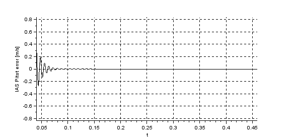
See PS.6 for the IAS pitot error, IAS is a step of 20 m/s at 0 s, after the transitory period IAS real = IAS pitot, so IAS pitot error is zero.
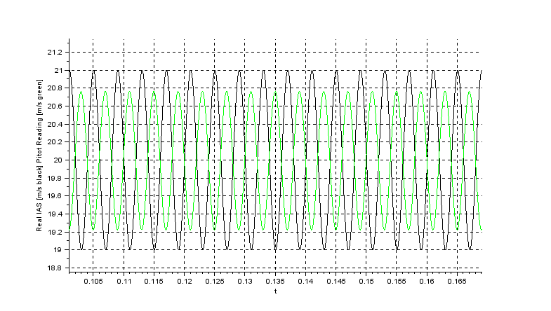
Now set to 250 Hz the input frequency, your simulation should result like that of figure PS.7.
To run the simulation issue the following Scilab commands
[f, m] =phasemag(repfreq(q,250))
Note that phase is -172° so input and output are almost opposite in phase.
By inspection of figure PS.7 max black value variation is 21-19,995 = 1,005, at the same time instant t=0,117 max green variation 20-19,222=0,778 so we have a magnitude of transfer function equal to 0,778/1,005=0,774 that is according to our attended value.
Make another run with the input set to124 Hz sine signal, use this command
[f,m]=phasemag(repfreq(q,124)
You should get 5.95 that is the ratio between output amplitude and input amplitude, and you should read the same values on the simulation plot.
You have the pitot math model, so you understand what frequencies will be distorted, if you integrate the pitot block into your air platform simulation you can determine if your instrument setup is suitable in any particular flight condition of your choice.
A strong conservative approach does not rely on pitot data if is expected to exceed the unitary gain band frequency, doing so you can trash every Pitot dynamic information and substitute the pitot with a unary gain block. Dynamic performance is useful when you eventually need high working frequencies, for example for a rotating head pitot setup. For my average application, I usually go in a conservative way.
References
[1] H. Tijdeman, “Theoretical and experimental results for the dynamic response of pressure measuring systems by H.Bergh and H.Tijdeman.” Unpublished, 1965 [Online]. Available: https://doi.org/10.13140/2.1.4790.1123