CFD Flow in a Pipe - Basic Air Data

cfd-flow-in-a-pipe_COVER

Computational fluid dynamics is a versatile and powerful tool, nevertheless it’s scarcely used in DIY applications. Nowadays there are some free CFD software at home maker disposal, the calculation power of personal computers is enough to reasonably cope with CFD design tasks.

There are many CFD commercial packages available, as well as a lot of well documented simulation cases, just to stay in topic have a look to the pitot simulation here. CFD commercial codes, and other needed software to complete the toolchain is not in typical DIY maker budget range, hence the numeric example will be carried out using the free and well proven package Elmer CFD.

At a glance, returning to our typical basic air data problem, CFD can calculate the velocity, pressure, temperature and density field for our given geometry and so derived standard defined aerodynamics parameters as the lift and the drag. With an adequate calculation power it’s possible to estimate position error for a particular aircraft and instrument.

For the sake of simplicity the problem solution with CFD techniques is split into six main subproblems that are defined here below; after general concepts a numeric example is inspected.

Goal of the example is to compare analytical results with CFD results.

All the files needed for the example Elmer CFD can be downloaded here.

CFD main phases

Preliminary study phase: It is necessary to study the problem analytically, in such a way the sought test cases are individuated. With the preliminary study done it is possible to individuate the assumptions and simplifications that can be acceptable. For example a simplification can regard a geometric complexity reduction or the decision to neglect thermal transfer equations, both the cases can yield to a dramatically reduction of modeling, meshing and simulation time. Study phase is fundamental to check simulation results.

Geometric modeling phase: Here a 3D or 2D model of the case to be simulated is drawn, no matter what software or format you use as long as it is easy to pass the data to the mesher software.

Meshing: Mesher must add simulation related information to our model, the model should be divided in regions and surfaces, for the mesh to be usable all the boundaries relevant to the physical problem must be identified. This features will be used during the simulation setup phase to define fluids, solids and boundary conditions properties. Mesher must also divide the simulation physical domain into a discrete grid, in a CFD problem the physical variables are calculated, for example, on the vertex of the grid. Unfortunately the accuracy of the simulation result is dependent on the mesh geometry itself. Choice of the grid dimension is not trivial and once again a preliminary study can give some information, for example if our simulation aim to study a boundary layer to have an estimation of layer thickness can aid to choice a proper grid dimension. Please have a look to this site to have a good introduction to the meshing.

Simulation setup and run: At this point you define in fine detail the properties of all the fluids, solids and boundaries and define what kind of solver you want to use during the simulation, incompressible flow, compressible flow, steady solution, dynamic solution heat transfer and so on. You must also define initial conditions, these are the values that variables take at the beginning of simulation, you can calculate or neglect such a values only if you carried out a good preliminary study phase. Numeric calculation phase, usually stop when the variation of the solution across successive iterations is less than a threshold value specified during setup.

Data visualization and post processing: Here you can visualize, physical values as speed, pressure and density as vector and punctual values. If you want the value of some derived physical quantity you can extract data and compute your derived value, for example you can calculate the flow rate over a surface integrating the velocity associate to this surface.

Solution validation: After a result as been reach is common to run again the simulation using different meshes sizes and shapes. The results with different meshes should be the same, after that also a more selective constrain on convergence should be applied. It’s to be noted that validation of the solution is reached if some analytical support is available.

Working example

Well, as CFD is a quite articulate topic, it’s better to check general concepts introducing a simple example. The example consist in a pipe of 0,1 meter diameter and long 1 meter. A certain amount of air at 20°C and 101325 Pa of pressure is blown into the pipe, with a constant speed over the inlet pipe section.

Preliminary study phase

As you know the interaction of air with the pipe walls will create a boundary layer, macroscopic effect is the velocity magnitude relation with the wall distance. As the flow pass through the pipe a variable speed profile along the pipe length is to expect, at least since the flow stream reach an Equilibrium.

Now that we have a well defined problem it’s possible to use common available bibliography like this notes online.

Our CFD case will be identical to those depicted in reference figure 8-8, whereas a common problem was chose it’s also available a closed form solution; a little investigation into the reference lead to focus on the equation 8-17 that state that fully developed velocity profile for a laminar flow into a circular pipe have a parabolic shape. In a fully developed flow region of our example pipe given pipe radius $R=0.05 \ m$ , average velocity $V_{avg}=0.1 \ m/s$ and defined r as the position on radius the axial velocity u(r) can be written as:

(P11.1) $\begin{equation*} $ u(r) = 2 \cdot V_{avg} \cdot \left( \frac{1-r^2}{R} \right) $ \end{equation*}$

Substituting our parameter values $0.2(1-r^2/0.05^2)$ that yields for laminar flow so Re<2300 should be verified.

To calculate Reynolds number the below fluid properties at operating temperature and pressure are used:

Name = "Air (room temperature)"
Reference Temperature = 20°C
v, Viscosity = 1.983e-5 Pas
Compressibility Model = Perfect Gas
Reference Pressure = 101325 Pa
rho, Density = 1.205 kg/m^3

Hence $Re=\rho \cdot D \cdot \frac{\displaystyle V_{avg}}{\displaystyle v} = 608$ , so it’s safe to assume laminar flow condition.

Geometric modelling phase

Tridimensional model of the pipe is just a 1m cylinder with 0.1 m of diameter; you can use the really powerful and free of charge freecad. Generated model is then saved as .stp format, like this.

After that is sufficient to launch the ElmerGUI and just open the .stp file.

Meshing

Into ElmerGUI geometric viewer set the mesh max h to 0.1 and min to 0.005; after apply the mesh the cylinder looks like the figure here below.

Figure PF11.1 – Cylinder, of course with opinable but easy to attain mesh

After meshing you will get three boundary surfaces and one volume as fluid, that in our case is air.

The three surface are exactly the inlet section, outlet section and the wall.

Simulation setup and run

ElmerGUI can be used to introduce every parameter or setting that I’ve used, anyway for your convenience the configuration for the simulation phase is contained in this case.sif file, it’s plain text so you can have a look into it.

Define the boundary conditions as per following table, an INLET with a constant velocity profile of magnitude 0,1 m/s, the OULET with a constrain on the velocity component along y and z axis that is zero and finally on the cylinder surface a WALL BC. Pay attention to assign the condition to the correct surface number, coordinates as following 1=x 2=y 3=z.

Boundary Condition 1
Target Boundaries(1) = 1
Name = "OUTLET"
Velocity 3 = 0
save scalars = logical true
Velocity 2 = 0
End

Boundary Condition 2
Target Boundaries(1) = 2
Name = "WALL"
Noslip wall BC = True
End

Boundary Condition 3
Target Boundaries(1) = 3
Name = "INLET"
Velocity 3 = 0
Velocity 1 = 0.1
Velocity 2 = 0
End

Define also the fluid properties as Fluid properties, from case.sif:

Name = "Air (room temperature)"
Reference Temperature = 20°C
Viscosity = 1.983e-5 mPa
Compressibility Model = Perfect Gas
Reference Pressure = 101325 Pa
Density = 1.205 kg/m^3

Assign this fluid to the “body” entity that represent simulation volume.

Initial state is set for the entire fluid volume, our initial state is an uniform axial flow field of 0.1 m/s magnitude at a pressure of 101325 Pa.

Set then the solver to search for a steady solution using only Navier-Stokes equation (no flux eq) You can note into sif file that ‘flowsolver’ solver is active, that solver integrate air velocity over the inlet boundary, just useful to check for the value of flow rate. Note also that simulation is setup to write the final step data into a file .vtu file.

Running the solver after iterations it converges as per figure P11.2

Figure PF11.2 – Simulation convergence history

After convergence, look for threshold into the setup section in case.sif file, have been reach it’s possible to check for the flow rate value. In detail in the solver output windows at the last iteration should read:

...
SaveScalars: -----------------------------------------
SaveScalars: Saving scalar values of various kinds
SaveScalars: Performed 1 reduction operations
SaveScalars: Found 3 values to save in total
SaveScalars: Showing computed results:
SaveScalars: 1: convective flux: flow solution over bc 1 9.420126351287E-004
...
ResultOutputSolver: Saving in unstructured VTK XML (.vtu) format
VtuOutputSolver: Saving results in VTK XML format
VtuOutputSolver: Saving to file: ./case0001.vtu
ResultOutputSolver: -------------------------------------
ElmerSolver: *** Elmer Solver: ALL DONE ***
ElmerSolver: The end

The simulation calculated flowrate is “flow over bc1”, a value of 9.4e-4 kg/s

Data visualization and post processing

As you already seen some data can be directly read in the simulation output screen, this possibility is quite comfortable during long simulation runs.

Anyway the final simulation step variables will be stored in case.ep file and case000.vtu

Example results can be visualized with the ElmerGUI integrated postprocessor VTK or, for example, with an external application that can handle .vtu files. Have a look to Paraview for a free well suited postprocess package that can handle .vtu files.

It is straightforward to setup tridimensional views and sections, see following figure for a view of velocity_x contour in a section view of pipe

PF11.3 – Velocity contours of a section view, inlet at the left side, outlet on the right side

Note on the above figure that in the inlet section the velocity have the attended constant magnitude, as expected the velocity profile evolves and at the outlet seem to be fully developed.

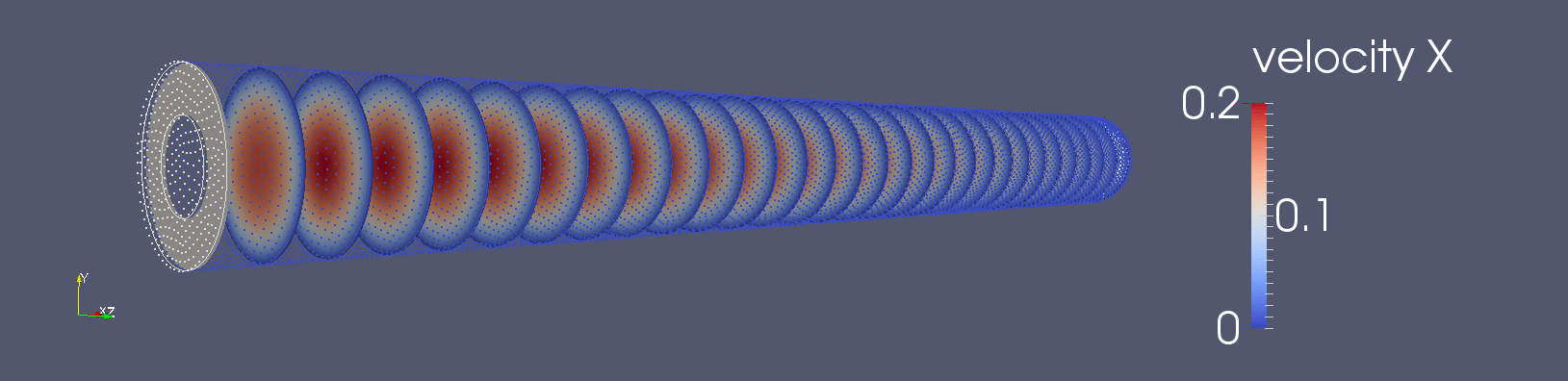
PF11.4 – Velocity plot with multiple slices with Paraview, inlet at the left side, outlet on the right side

Paraview can also handle multiple views and data from parallel processing runs. With this postprocessor is easy to retrieve simulation data and setup custom data filters, for example in many cases there in no need to configure elmer to write to file common simulation values; for example in the following figure the velocity profile is directly selected and plotted into Paraview.

PF11.5 – Venturi velocity profiles at different location, Paraview Solution validation

At glance our problem have been defined with the following parameters:

Geometry of cylindric pipe
L=Pipe length 1m
D=Internal diameter of pipe 0.1m

Fluid properties, from case.sif:

Name = “Air (room temperature)”
Reference Temperature = 20°C
v, Viscosity = 1.983e-5 Pas
Compressibility Model = Perfect Gas
Reference Pressure = 101325 Pa
rho, Density = 1.205 kg/m^3

Fluid axial velocity is $V_{avg} = 0.1 \ m/s$
$Re = \rho \cdot D \cdot \frac{\displaystyle V_{avg}}{\displaystyle v}=608$ : Re<<2300, laminar flow

At the input section mass flowrate can be written as:

(P12.2) $\begin{equation*} \begin{align*} \(q_m &= q_v \cdot \rho \\ &= V_{avg} \cdot \pi \cdot D^2/4 \cdot \rho \\ &= 9.4 \ e-4 \ kg/s \end{align*} \end{equation*}$

Good news are that calculated flow rate is the same that previously simulated flow rate, starting from this result is necessary to have an evidence that simulated velocity profile is that predicted by eq P12.1. Simulation was setup on purpose to save velocity values along the inlet section radius, you find this data into g.dat file, into profile compare spreadsheet you find the figures. The validation idea is to plot simulated values against calculated values, you can see the results in the following figure.

F11.6 – Velocity profile comparison, evident agreement between two methods

By inspection of figure it’s safe to say that there is an evident match, it’s far more evident in the following figure that plot simulated velocity deviation from the ideal case.

F11.7 – Absolute deviation from ideal case