
Figure 1 – Falling Apple
The value of telemetry data can be enhanced by the application of basic estimation and modeling techniques. In most real-life cases, even in the simplest systems, it is either too expensive or impossible to measure every relevant variable. Thus, one needs to make do with a reduced number of sensors, which are also quite noisy.
In these articles, I will present a complete application example in the form of a miniseries. The core idea is to investigate the performance of an algorithm that uses data from accelerometers and a GPS to enhance altitude measurement. That method should be implementable on mobile devices and can improve the previously implemented altimeter. The very same algorithm can be used to post-process primary flight telemetry data.
Article summary:
- Introduction post: the state estimation problem and state observer;
- Altitude measurement enhancement with an accelerometer, performance evaluation;
- Altitude measurement enhancement with accelerometer and GPS data, performance evaluation;
The working code will be posted where needed.
To use telemetry data in a meaningful way, it is necessary to have a mathematical model of our physical system. One possible representation is the state space representation.
A continuous linear system is represented as:
![\[\begin{array} {rcl} \boldsymbol{\dot{x}}(t) & = & \boldsymbol{A}(t)\boldsymbol{x}(t)+\boldsymbol{B(t)}\boldsymbol{u}(t) \\ \boldsymbol{y}(t) & = & \boldsymbol{C}(t)\boldsymbol{x}(t)+\boldsymbol{D}(t)\boldsymbol{u}(t) \end{array}\]](http://www.basicairdata.eu/wp-content/ql-cache/quicklatex.com-0404e687919792b5cc7cade5c8565126_l3.png "Rendered by QuickLaTeX.com")
Bold notation indicates vectors or matrices. All quantities are time dependent. This is a fully deterministic model, whose the mathematical representation is a set of ordinary differential equations.
 is the vector containing the physical system state variables,
  represents the output variables and
  is the system input. All the other matrices describe the relationships between those variables.
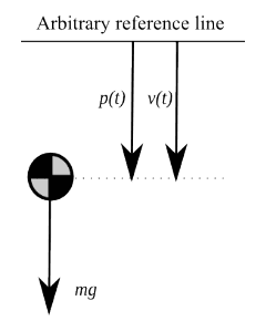
Figure 2 – Model definition
However, in our example case, we can make some assumptions towards the simplification of the system:
![\[\begin{array} {rcl} \boldsymbol{\dot{x}}(t) & = & \boldsymbol{A}\boldsymbol{x}(t)+\boldsymbol{B}\boldsymbol{u}(t) \\ \boldsymbol{y}(t) & = & \boldsymbol{C}\boldsymbol{x}(t)+\boldsymbol{D}\boldsymbol{u}(t) \end{array}\]](http://www.basicairdata.eu/wp-content/ql-cache/quicklatex.com-a401ce86e6e15040095e9f2f297d7c35_l3.png "Rendered by QuickLaTeX.com")
Now system matrices are time independent. Last set of equations is a model for a Linear Time Invariant system. If  has a dimension of
  , then we say that the system has a dimension of
  . To better explain the state space representation I’ll use a simple mechanical system. Suppose we need the mathematical model of a falling apple.
To simplify the math, suppose the falling apple is not rotating. Assume also that the apple is moving through the void; thus aerodynamics are not involved. The apple will fall vertically.
The system dynamics can be described using Newton’s second law:
![\[\boldsymbol{F}=m\boldsymbol{a_z}= m\boldsymbol{g} \rightarrow a_z=g\]](http://www.basicairdata.eu/wp-content/ql-cache/quicklatex.com-70fa3e623e9f960d1607a438a01ec5e0_l3.png "Rendered by QuickLaTeX.com")
Using standard notation we can write:
![\[\begin{bmatrix}\dot{p} \\ \dot{v} \end{bmatrix} =\begin{bmatrix}0 &1 \\ 0& 0 \end{bmatrix} \begin{bmatrix}p \\ v \end{bmatrix}+ \begin{bmatrix}0 \\ 1 \end{bmatrix} g \]](http://www.basicairdata.eu/wp-content/ql-cache/quicklatex.com-e0729e51451b080eb99fbb1f8181483e_l3.png "Rendered by QuickLaTeX.com")
Note that we have chosen not to model the output . It is not necessary in this example.
You can observe that such a model is not entirely realistic. According to it, the apple will fall to infinity with a uniformly accelerated motion. As in most occasions, the model is accurate only around specific conditions: the previous apple model is correct for a shortfall in the void before the apple hits the plate.
Commonly the model of a phenomenon is not linear but can be considered linear around predefined state variables values. That’s one reason why linear models are useful for real-world modeling systems.
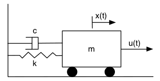
Figure 3 – Mass-Spring-Damper System
Let’s move over to a more complex system and examine a complete numerical example. The system is composed by a mass, a spring and a damper. It is a classic literature example, for which you can find a description in this link. Download in these links the Scilab and Matlab script files for the Mass-Spring-Damper example.
Let’s suppose that we want to know the position and the speed of the mass with a single position sensor. I know it’s simple to find the solution; however the systematic solution that I will show here can be used on more complex systems. In particular it will be used on the inertial navigation system which will be presented later.
State estimation consists of getting the values of state variables without measuring them. We will achieve such a result with the use of a state observer.
The main working hypothesis is that the physical system is correctly modeled, in this case, as an LTI system of known  matrices. The model of the system is supposed to describe precisely the physical system behavior.
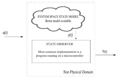
Figure 4 – Estimation layout
We do not need to identify the parameters or the order our system, but we are only looking for the state space variables values. That the main idea is to get measurement values from a limited set of sensors and obtain the observed state estimation. To that goal, we will use a Luenberger Observer architecture, an estimator which is a closed loop state observer.
Estimated variables will be indicated with the circumflex or hat notation.
Returning to the mass-spring-damper system the continuous time estimator will be described by the following system of equations. The only available sensor measurement is the mass position. The estimator gain is contained in the  matrix.
![\[\begin{array}{rcl} \boldsymbol{\dot{\hat{x}}}(t) & = & \boldsymbol{A}\boldsymbol{\hat{x}}(t)+\boldsymbol{B}\boldsymbol{u}(t)+\boldsymbol{L}(\boldsymbol{y}(t)-\boldsymbol{\hat{y}}(t)) \\ \boldsymbol{\hat{y}}(t) & = & \boldsymbol{C}\boldsymbol{\hat{x}}(t) + \boldsymbol{D}\boldsymbol{u}(t) \end{array}\]](http://www.basicairdata.eu/wp-content/ql-cache/quicklatex.com-88731448c580543eab6a87124e30e1af_l3.png "Rendered by QuickLaTeX.com")
Given spring constant  , damping constant
  and body mass
  , we get:
![\[\begin{array}{rcl} \boldsymbol{A} & = & \begin{bmatrix}0&1 \\ -k/m&-c/m \end{bmatrix} \\ \boldsymbol{B} & = & \begin{bmatrix} 0 \\ 1/m \end{bmatrix} \\ \boldsymbol{C} & = & \begin{bmatrix} 1 & 0\end{bmatrix} \\ \boldsymbol{D} & = & \begin{bmatrix} 0\end{bmatrix} \end{array}\]](http://www.basicairdata.eu/wp-content/ql-cache/quicklatex.com-ba33fe2af9d73450917ddf3e10c3fd26_l3.png "Rendered by QuickLaTeX.com")
For presentation purposes, in the provided script files, the simulation state starts from [1 ; 0] and the system input is set to zero. You can see how the position oscillates with time and how well the observers track the velocity state.
Before the use of an observer it’s necessary to check the observability matrix rank. If the rank is equal to the system order, then it is possible to observe every state of the system. For our system ![O=[C;C*A]](http://www.basicairdata.eu/wp-content/ql-cache/quicklatex.com-0dd0c56363fc125b7749304214a1f5e4_l3.png "Rendered by QuickLaTeX.com") and the rank of
and the rank of  is two, equal to the rank of our system which is also is two. Hence the system is entirely observable (command rank(O)). Another property that should be checked is system stability. For now, we will avoid dealing with unstable systems. By issuing the command spec(A) in Scilab or eig(A) in Matlab we get the system eigenvalues, which are also called poles of the system. If the real part of every pole is negative, then the system is stable. In our case, the eigenvalues are a complex conjugate pair -0.1 ±0.53i, and the system is stable.
With complex eigenvalues, the state variables trajectories will oscillate when moving from one stable solution to another.
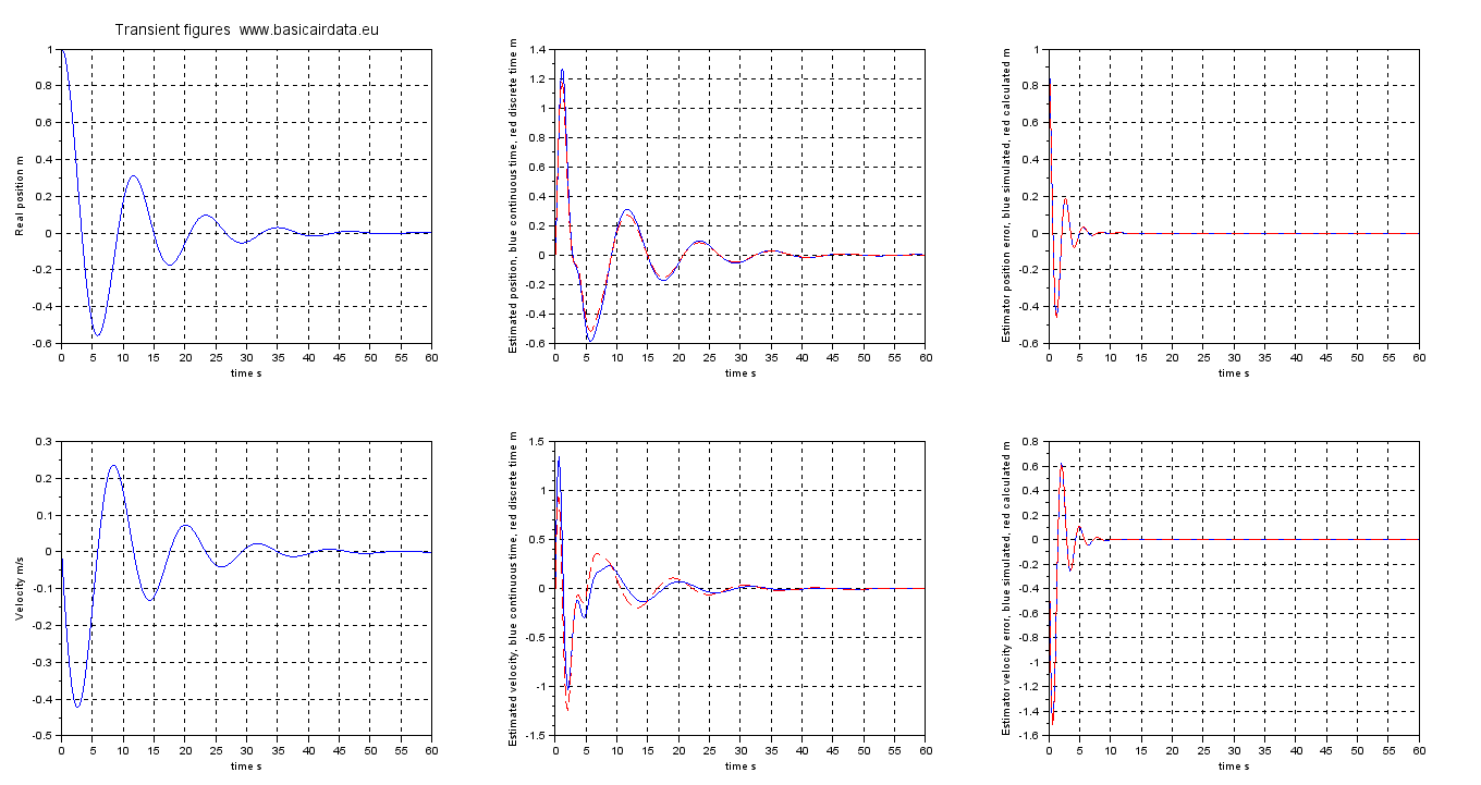
Figure 5 – Time response of system and state observer
This behavior is evident in the plots of figure 5.
If we define the tracking error as  we get:
![\[\boldsymbol{\dot{e}}(t)=(\boldsymbol{A}-\boldsymbol{L}\boldsymbol{C})\boldsymbol{e}\]](http://www.basicairdata.eu/wp-content/ql-cache/quicklatex.com-0e015ff95754eb04f7ae325501af5532_l3.png "Rendered by QuickLaTeX.com")
Hence, the error dynamic response is directly defined by matrix. The poles of  should be stable to have a usable estimator.
In our example, we get the stable complex poles -0.6 ±2.1i, which generate an oscillating, but stable, trajectory that is evident in figure 5.
With the dynamic of the error so well defined, it is possible to shape the response, for example, with a pole placement method. If we want two real poles at -5, we can issue the Scilab command:
Lt=(ppol(A',C',[-0.5 ;-0.5]))'Afterwards, we can check the closed loop poles values with spec(A-Lt*C). In Matlab the commands are:
Lt=place(A',C',p).'
eig(A-Lt*C)
After this little introduction, we have the tools to understand the altitude measurement system enhanced with accelerometers and GPS. A key point to our further analysis will be the characterization of the error variance of the state estimation.
We will quickly examine one degree of freedom inertial unit. With such a unit it will be possible to measure altitude variations directly. Accompanying scripts for Matlab and Scilab are provided for download.
The use of inertial units requires considering the mounting position, as explained in these articles.
Let’s pretend we want to measure the altitude variation of our aircraft using the measurements from an accelerometer. To obtain an initial value, we define an arbitrary, zero-reference position and an altitude direction. The altitude value from the reference is (t), velocity is (t) and acceleration (t) From now on, assume that the acceleration measurements are always aligned with axis, which is as if we modeled a simple flat fall, but this hypothesis allows us to focus on a specific problem. In a real-world case, other measurements from the rest of the axes of the inertial unit should be used to get the correct acceleration value.
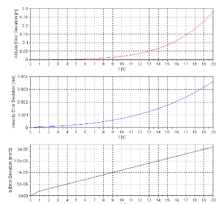
Figure 6 – Error deviation Vs time for example system, initial variance set to zero
The kinematic equations of our system are:
![\[\begin{array} {rcl} \dot{z}(t) & = & v(t) \\ \dot{v}(t) & = & a(t) \end{array}\]](http://www.basicairdata.eu/wp-content/ql-cache/quicklatex.com-c82a951c8ff2ff490033bd88968e034c_l3.png "Rendered by QuickLaTeX.com")
The measurement system cannot be considered deterministic, since it is prone to measurement errors. We model the accelerometer output as:
![\[\hat{a}(t)=a(t)+b(t)+\mu_a(t)\]](http://www.basicairdata.eu/wp-content/ql-cache/quicklatex.com-85faf0e1222a2152b65bdabd81b5cf81_l3.png "Rendered by QuickLaTeX.com")
 term represents the random walk of the sensor (Paragraph 3.2.2) and
  is a Gaussian white noise with given variance
  . The latter term aggregates different kinds of uncertainty sources such as thermal noise.
Random walk noise is defined as  where
where  is Gaussian with given
  . The average value of is zero.
It is interesting to note that while a constant accelerometer error  (Paragraph 4.2.1) leads to an error term equal to
  , that constant error can be eliminated with an accurate calibration, hence it is not that interesting to take into account and examine.
If we wanted to reconstruct the aircraft altitude based solely on the accelerometer readings and the zero initial altitude assumption, the observed altitude would be:
![\[\begin{array}{rcl}\dot{\hat{z}}(t) & = & \hat{v}(t) \\ \dot{\hat{v}}(t) & = & \hat{a}(t) \end{array}\]](http://www.basicairdata.eu/wp-content/ql-cache/quicklatex.com-c7709163fffb7e35356f77107a6ecf18_l3.png "Rendered by QuickLaTeX.com")
Navigation equations are [1] [2]:
![\[\begin{array}{rcl} \boldsymbol{x} & = & \begin{bmatrix} \hat{z}\\ \hat{v}\\ \hat{b} \end{bmatrix} \\ \dot{\hat{z}}(t) & = & \hat{v}(t) \\ \dot{\hat{v}}(t) & = & \hat{a}(t) \\ \dot{\hat{b}}(t) & = & 0 \end{array}\]](http://www.basicairdata.eu/wp-content/ql-cache/quicklatex.com-d38f3295a7b29366954b6100d61960ed_l3.png "Rendered by QuickLaTeX.com")
As we are interested in error dynamic we define a new error state variable  :
:
![\[\delta\boldsymbol{x}(t)=\boldsymbol{A}\delta x(t) +\boldsymbol{B}\begin{bmatrix}\mu_a \\ \omega_b \end{bmatrix}\]](http://www.basicairdata.eu/wp-content/ql-cache/quicklatex.com-dbdf85cb24e9c6f3d33046d0227c6821_l3.png "Rendered by QuickLaTeX.com")
General definition of process noise covariance for a continuous system is 
Defining 
The state error covariance is [2] :
![\[\boldsymbol{P}_x(t)=\boldsymbol{\Phi}(t)\boldsymbol{P}_x(0)\Phi^T(t)+\int_0^{\tau} \boldsymbol{\Phi}(t)\boldsymbol{B}\boldsymbol{Q}\boldsymbol{B}^T\Phi^T(t)d\tau\]](http://www.basicairdata.eu/wp-content/ql-cache/quicklatex.com-2da71416eb2f0fcf383dfee8c49c4f6d_l3.png "Rendered by QuickLaTeX.com")
This is one of the rare cases where solution can be calculated in a closed form, terms with subscript 0 denotes initial value.
![\[\begin{array}{rcl} P_P(t) & = & (P_{p0}+P_{v0}t^2+P_{b0}t^4/4)+(\sigma^2_{\omega_v}t^3/3+\sigma^2_{\omega_b}t^5/20) \\ P_v(t) & = & (P_{v0}+P_{b0}t^2)+(\sigma^2_{\omega_v}t+\sigma^2_{\omega_b}t^3/3) \\ P_b(t) & = & P_{b_0}+\sigma^2_{\omega_b}t \end{array}\]](http://www.basicairdata.eu/wp-content/ql-cache/quicklatex.com-0511214aa7d089e44a9d161b18bca018_l3.png "Rendered by QuickLaTeX.com")
Let’s set  or velocity random walk to a value of
  ,
,  and
and  .
.
As expected and plotted in Figure 6, the use of an inertial sensor alone leads to an unacceptable altitude error in a few seconds. In the next post, this inertial unit will be coupled with a GPS to provide an enhanced measurement.