Measuring airflow with Pitot tube

Figure 1 - Sectioned pipe and flowing fluid

Single point and multipoint airflow measurement are possible with the ADC.

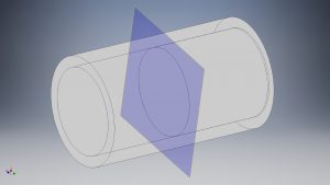
In this article, we estimate the flow rate value at a circular pipe section via n multiple velocity measurements. Although this article doesn’t reflect any particular technology, the reader can imagine that velocity measurements themselves are carried out with a Pitot tube or with a Pitot rake placed at the section in question. There are different industrial standards that cover the topic, such as the ISO 3966: Measurement of fluid flow in closed conduits – Velocity area method using Pitot static tubes. We will not follow any particular standard. Still, those standards are interesting readings.

We want to calculate the volumetric flow rate, $Q$ . The volumetric flow rate is the volume $\Delta V$ that flows across a predefined surface in an arbitrary interval of time $\Delta t$ , $Q=\frac{\Delta V}{\Delta t}$ .

Refer to Figure 1. A section perpendicular to the pipe axis defines a circular surface of area $s$ . On the assumption that the axial velocity at every point of the section is constant and equal to $V_c$ , then $Q=V_c\cdot s$ . An animation of the system at hand can be seen in the following video.

However, in the real world, the velocity is not constant across the section. The interaction of the fluid with the pipe surface generates a non-negligible velocity gradient. For axial flows, it stands that $Q=\int v(x,y,)dt$ . Bibliography comes handy and we will assume a power-law velocity profile. With this model, we will build a numerical model, which represents the pipe and the flow rate which we will measure. The real-world pipe is replaced by a numeric simulation. The commonly used model does not separate the viscous sublayer nor the transition layer; it is discontinuous at the surface of the pipe and on the symmetry axis. Since we are not treating a particular real-world case we’re not concerned about the uncertainty introduced by the power-law model. Details about the viscous sublayer and the transition layer can be found at this link.

We end up using a fully developed turbulent axial flow model at high Reynolds number. The viscous layer is expected to be thin in typical cases (thick like a hair) and it is not calculated in this example. You can find a Scilab script in this file that will calculate the power-law velocity profile for you. The result is visible in the next figure.

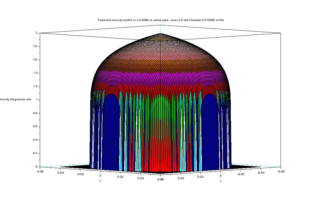
Figure 2 – Velocity profile, power-law approximation

The resulting velocity profile is dependent solely on the distance from the axis. You can see that the velocity gradient, as expected, is high near the pipe wall and low along the center line.

Now it is time to measure the flow rate. Refer to Figure 3. We assume having access to velocity measurements at $n$ stations. Each station is at a different distance $r(n)$ from the pipe center line. For the sake of simplicity, we divide the radius in $n$ equal segments. For each segment, we measure the velocity $v(n)$ at its midpoint.

Figure 3 – Velocity measurements stations

We make the assumption that the velocity remains constant along each segment of the pipe radius and, by extension due to axial symmetry, over the whole corresponding annular ring. The total volume that passes through the ring surface is the product of velocity with the annulus area. Iterating the calculation for all the segments we calculate the volumetric flow rate as

$Q=\sum_{i=1}^n v(n)\pi(r_{ext}^2(n)+r_{int}^2(n))$

, where

$i$ is the annular ring index
$v(n)$ is the velocity of $i$ ring
$r_{ext}$ is the outer ring radius of $n$ ring
$r_{int}$ is the inner ring radius of $n$ ring

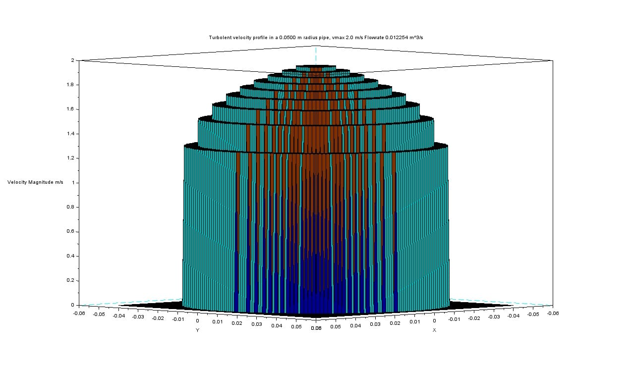
Figure 4 – Velocity profile reconstructed with 10 different measurements

Figure 4 visualizes the velocity profile as reconstructed by our measurements. It is evident from the profile steps that we have a coarse approximation. There is a simple way to get better flow rate measurements: we can use the model to calculate the velocity profile within each annulus. In such a way, using our simulation data, we will get exactly the flow rate produced by our reference model. Driven by this result, we can even try to use only the data from one single measurement, for example at the center line. Doing so we will get the very same result predicted by our reference model. Unfortunately, the effective accuracy is constrained by the ability of the model to capture the real world. For that reason, in actual applications, the overall accuracy should be expected to be higher when using multiple simultaneous measurements rather than model interpolations. But let’s leave this problem to the professionals.

In this article, we have explored the basics of volumetric flow rate measurement with the velocity-area method. Experimental data can be retrieved with a simple ADS.

Measuring airflow with Pitot tube

0 Comments

Leave a Reply Cancel reply