This is a tutorial like article about the CFD simulation of a classical, Von Kàrmàn vortex street example. Some basicairdata instruments, as angle of attack vane, can be affected by vortex wake.
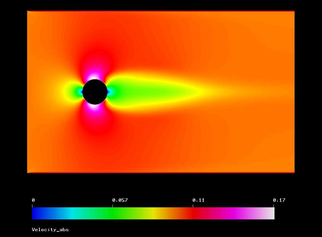
Video V25.1 Preliminary simulation output
The tutorial-like material will be referred to the following, free to download and to use software :
- 2D Sketching,Freecad, Draftsight
- Mesher, prepocessor Salome
- FEM engine, Elmer CSC
- FEM postprocessor, Paraview
The article will follow this scheme
- Sketching of the simulation layout
- Meshing of the simulation domain
- Non steady simulation run 1
- Considerations on the step-time and simulation run 2, example of bad convergence due to poor step-time choice
- Visualization of results and video production
Problem and CFD domain definition
Each object invested by airflow generates a wake. Basic air data instruments can be fooled by wakes, which is directly translated into poor measurement performances. In this mini-series we proceed with a concise presentation of the phenomenon and an introductive tutorial to CFD simulation. As main example we will use a Von Karman Vortex Street, a good article on the Street dimensions is downloadable here.
Von Karman Street is a phenomenon that can be observed in nature. Below a wake generated by Guadalupe island.

Figure P.35.1 Natural Von Karman Street, Retrieved from this site
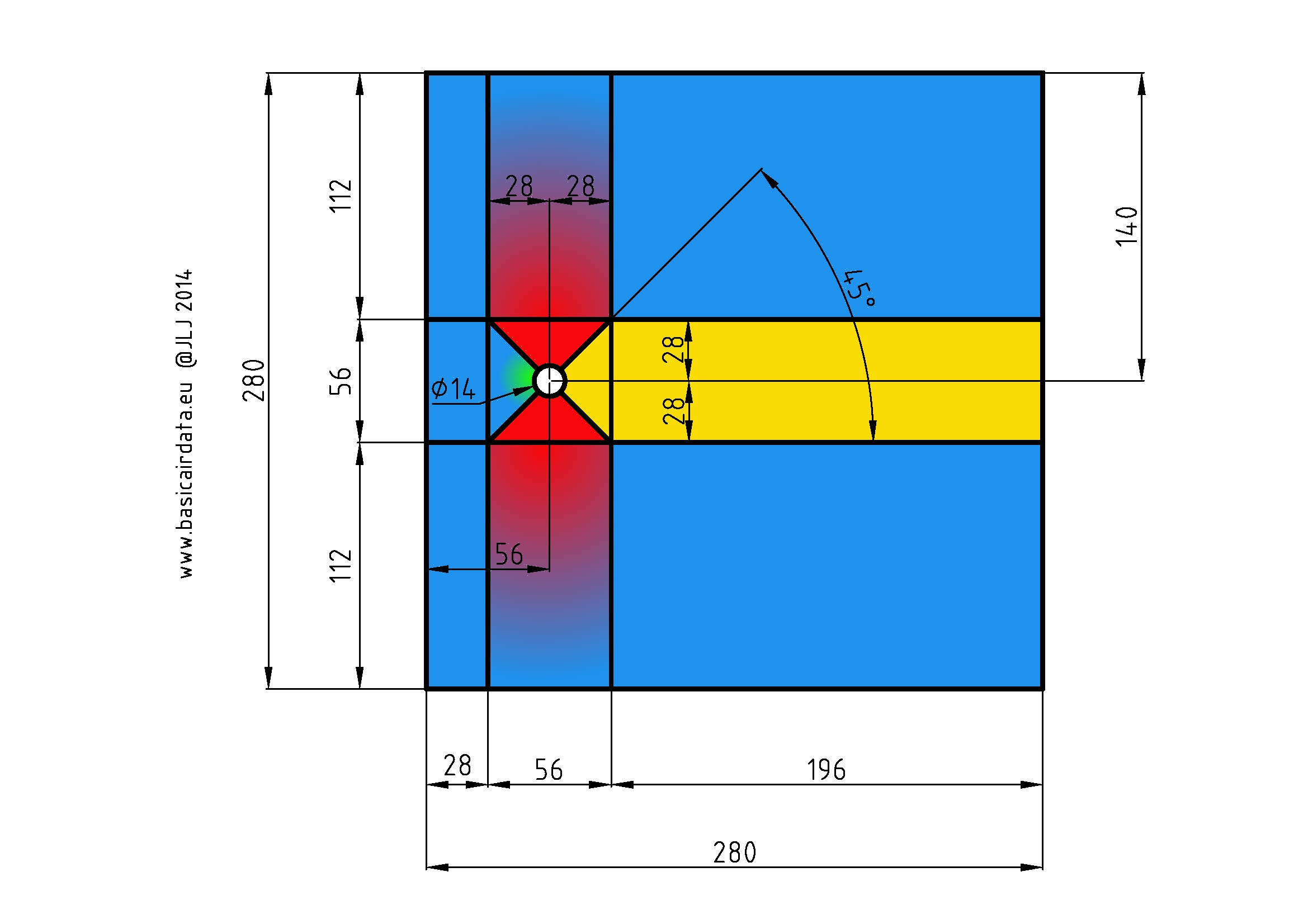
In the picture you can see how a constant speed airstream over an island lead to the formation of a periodic vortex wake in the clouds. Our experimental layout will be composed by a simple round bar of radius \(a\) immerged in to an airstream. A bidimensional numerical simulation is carried out; we simulate the plane that sections the bar along the radius plane. The general layout for the simulation is depicted in the following picture.

Figure P.35.2 General simulation layout
During the simulation the ISA standard conditions are assumed for the air
$$P_{air}=101325Pa$$
$$T_{air}=288,15°K$$
$$\rho_{air}=1,225kg/m^3$$
$$\mu_{air}=1,79e-5Pas$$
$$\gamma=C_p/C_v=1,4$$
$$M_{air}=28,96e-3 kg/mol$$
$$R=8,3145Jmol^{-1}K^{-1}$$
$$R_{air}=\frac {R}{M_{air}}=287,1 Jmol^{-1}K^{-1}$$
The air is modeled as incompressible, that is a fair hypothesis as long as the velocities magnitudes are less than \(0,3M\). Mach number, for ideal gas case, is \(M=\sqrt{\gamma R_{air}T}= 340.3m/s\)
Then 0,3M=102 m/s, we take care to use airspeeds \(U\) well below this value.
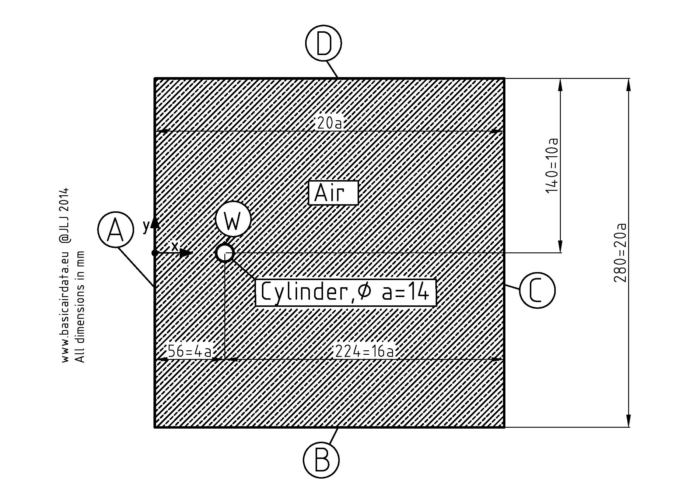
Consider the simulation boundaries. At the boundary A, B and D the airflow is directed along the \(x\) axis and have a known \(U_x\) speed. The constraint at the boundary C is that \(U_y=0\). Along the cylinder wall W the constraint is that speed along x and y axis is equal to zero.
The simulation domain dimensions have impact on the simulation performances and reliability; let’s shortly comment how they have been chosen. If we set the boundaries B and D y velocity component along to zero then we risk to modify the simulation behaviour; we will see how to set alternatively a pressure along the boundaries. Refer to the following figure that considers only the steady part of a inviscid flow around a cylinder. Our simulation considered the viscosity of the air, nevertheless a comparison with the inviscid analytic solution point out the velocity field modification around the bar.

Figure P.35.3A The streamlines of the flow over a circular cylinder of radius a

Figure P.35.3B Flow over a circular cylinder of radius a. Image from this link
As you note from the precedent figure the component along y axis at an arbitrary distance from the center of the cylinder is not equal to zero. The eq.11.60 enable us to quantify how far we are from the \(U_y=0\) condition. The flow potential formula along streamlines indicates that we must be at the infinity to obtain a zero value for the second term of 11.60, a perturbation in the flow pattern will be perceived all over the plane. Using \(10a\) as y coordinate and\( x=0\) we get a deviation from the ideal case of 1/100. That is a good guess value for the value of distance between the bar center and the top and bottom boundaries. Same reasons yields to choose \(4a\) as the distance between the left boundary and the bar center. If the simulation boundaries are too close to the cylinder the numerical result can be invalidated; look at the following figure, the boundaries are too close and the velocity profile is clearly modified.
P35.4 Boundaries too close to the cylinder, velocity profile is sudden modified next to the boundary
In some occasion, as turnaround, is preferred to simulate a closed geometry and set the B and D boundaries as wall; that is really similar to a wind gallery setup.
Now it’s necessary to choose a value for airstream velocity. Wake behavior change with Reynolds number, have a look to the following figure. The accuracy of shown Reynolds numbers is not relevant.

P35.5 Different wake behaviors in function of Reynolds number. Retrieved here
We chose to go for a Reynolds number of 151 to get a slighty turbolent wake.
Velocity of airstream will be set to \(U_x=\frac{Re\mu}{\rho a}=0,157m/s\)
Periodic wakes have been studied by Strouhal , in particular the vortex formation behind a circular cylinder (Have a look for example to Blevins, R. D. (1990) Flow-Induced Vibration, 2nd edn., Van Nostrand Reinhold).
Strouhal number is defined as \(Sr=\frac{f_{vortex}a}{U_y}\), it give a relation between frequency of vortex generation and airstream velocity. Strouhal number should be determined by experiments, from bibliography[Blevins, R. D. (1990) Flow-Induced Vibration, 2nd edn., Van Nostrand Reinhold Co, cited also here] at Re=151 Sr should be bounded between 0,15 and 0,22.I take a value equal to 0,18 then \(f_{vortex}=2 Hz\)
This post is the third part of the Von Karman Vortex Street tutorial, precedent article in this link.
Within this post practical procedures for the domain drawing are introduced. Along the article the used softwares are DraftSight and Freecad. All the necessary files are linked along the article.
In the precedent post have been defined the layout and dimension of simulation domain. For numerical simulation is needed to divide the domain in a mesh, or grid. There are many different ways to mesh the domain and there is also the fascinating alternative to use an adaptive mesh, that last option uses a self-modifying mesh to achieve the best results. Right now is important to stress on the fact that we should consider the mesh type during the domain drawing phase, an accurate drawing phase will ease the meshing.
Among the different type of meshes is chosen the Quadrilateral. Quadrilateral mesh is a structured collection of four sided polygons or cells. The mesh is structured so it’s possible to set exactly how the mesh will look like. Of course an unstructured mesh will do the same job; in fact for the preliminary simulation a triangular unstructured automatic generated mesh was used, indeed I should say a fast solution. First impact of the use of quadrilateral mesh is that we need to divide our domain in subdomains with exactly four sides. If a region have not exactly four sides cannot be meshed with quadrilateral cells.
For best results the mesh polygons should be aligned with the flow, that condition cannot be satisfied all along our transient simulation, in particular in the wake region. That is not a problem as long as the cell size is small enough. More details on the topic in the post about meshing, the important thing to focus on is to verify that different cells sizes are needed along the domain in function of flow condition.
Let’s proceed to the domain drawing. We use Salome as mesher a domain file format compatible with this software is necessary, we chose step file format. We use two software in sequence because we generate a DXF with DraftSight and then we convert it to Step format with Freecad.
DraftSight operations are basic, launch the software and draw line by line the partitioned domain shown on figure F36.1. Draw all your segments using as length the dimension in millimeters, in such a way, with default setup for the software tool chain, the mesh imported into Elmer CSC will have the correct dimensions in meters. Have a look to the following video for a complete description of the drawing and conversion phase.
V36.1 Video on the drawing procedure, including conversion to step file format
Right now you should have one DXF file and one STP file really similar to these files downloadable here.
Mesh
Video 1 Tutorial of meshing procedures
Video edit procedures in Paraview are shown.
Some mail arrived during the tutorial posting, based on that feedback I decided to reduce the calculation power needed to simulate the examples files.
You find all the needed Elmer project files into “Vonkarmanforvideo.zip” archive.
All the required files are contained in the archive, “case.ep” and vtu simulation output files have been excluded to minimize archive dimension.
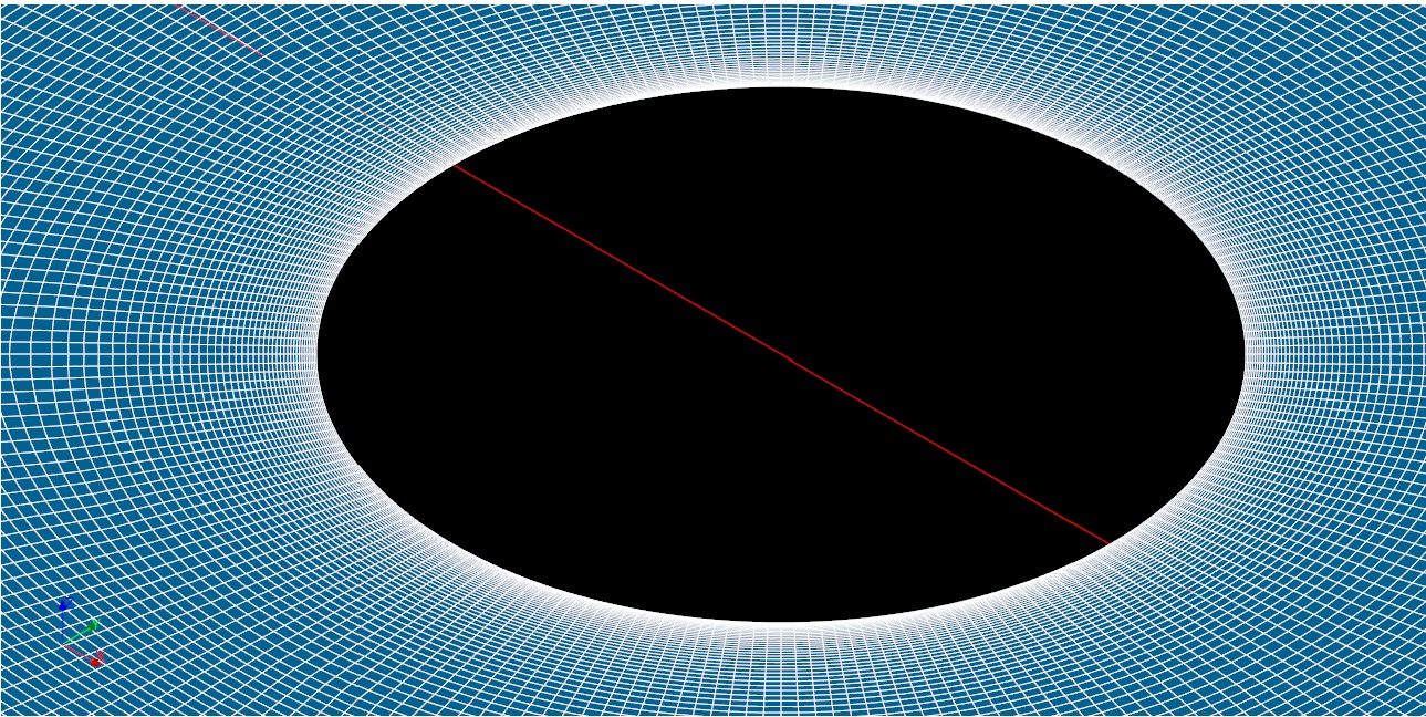
Mesh has been generated into Elmer GUI using the internal mesher. You can appreciate how coarse is the mesh in the following figure. Simulation is contained in a 1,6mx0.6m rectangular surface, the cylinder is set to 0.14m diameter, geometry dimensions of cylinder have been increase to ease simulation convergence. Of course if quantitative solution is needed the mesh should be refined.
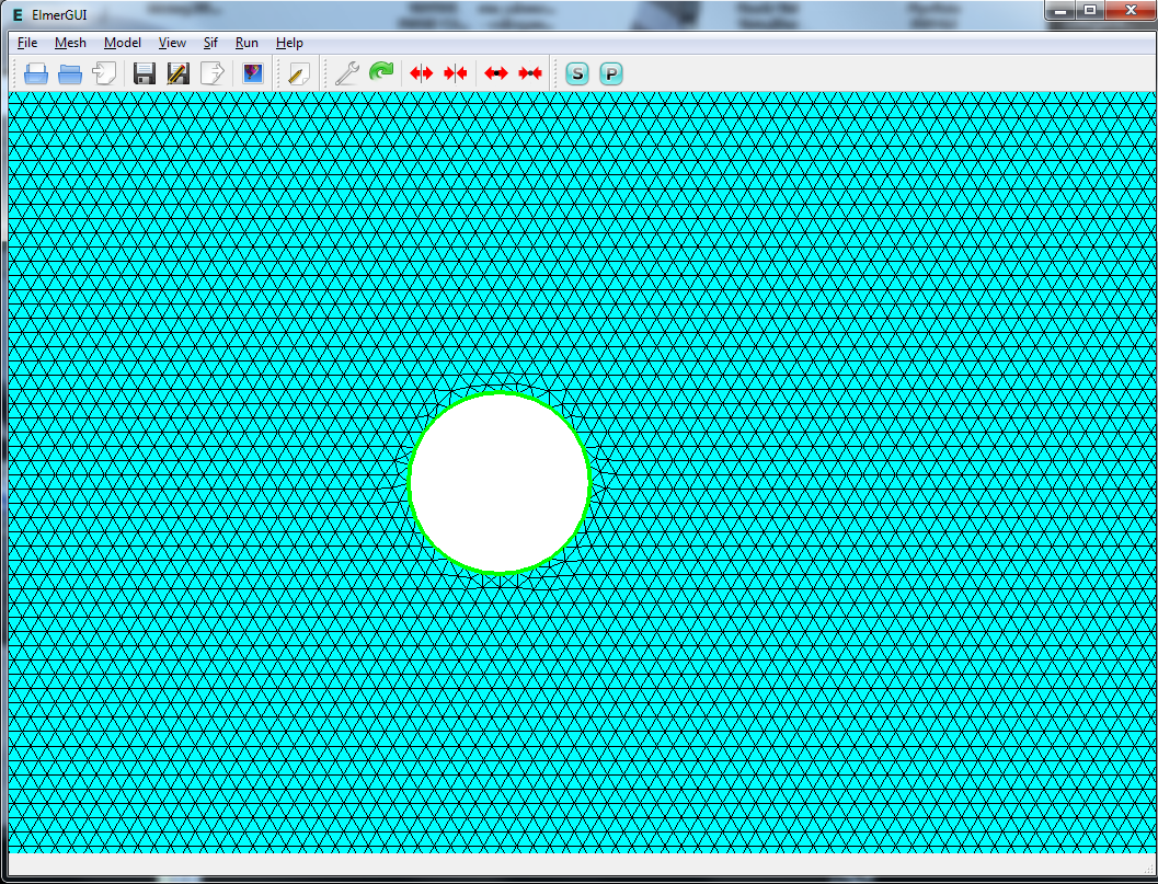
Figure 43.1 Simulation Mesh, elements have 10 mm side length.
Simulation is set to transient with 1500 steps of 5e-3 seconds; respect to precedent case the simulation is not any more in an open domain but is now limited by two walls. Simulation have not special configuration issues, you can read all the parameters into “case.sif” ASCII file; Elmer default parameters work fine.
Remember to enable simulation output, in this way simulation steps will be saved in a collection of vtu files that set of files will be used later into Paraview for video production.
Simulation time step should be chose by user. There are not broadly accepted rules to select simulation step size. A rigorous approach can be followed but is neither practical nor easy. Many CFD users rely on the Courant condition. That is a sensitive topic, results are variable in function of simulation equations involved. For a Navier-Stokes equation can be acceptable to impose \(C<1\); That topic should be treat by its own, for our example tutorial that will not harm.
To follow this approach let’s set \(C=1=2\frac{tV}{u}=2\frac{t}{10e-3}\) then we get a time step \(t=5e-3s\)
Another approach can be those of reuse results from bibliography, in our particular case we need an approximate evaluation of the phenomenon dominant timescale. On purpose we use and approximation of expected vortex sheed frequency. Strouhal approximate number for our simulation is
Approx \(Re= 1700\) hence \(St=0.2\) and \(f=1.4 Hz\)
As a heuristic rule for every simulation, transport equation dominant, we need to have at least two orders of magnitude or more time samples of the phenomenon. Using our parameters that lead to \(t=7e-3s=\frac{1}{100f}\).
At this level of accuracy is sufficient to have a reasonable initial value. To validate the choice of time step is necessary to run different simulations with different time steps values, that topic will not be treated here. In our case if the time step is to big then we will not see vortex at all in the simulation results.
After the simulation run go to Paraview and load vtu case files then load “Solidmodel.stl”
Set the properties of “Solidmodel.stl” as per following values
Translation 0,5 0 -0,2 Scale 0,009 0,009 0,009 orientation 0 0 90
Now you can save the simulation animation
The video of the Paraview procedure is here below.