Pitot Correction for Position and Angular Rates

Figure 1 – A plane flying at high AOA. Notice the airboom vanes

Pitot probes are widely used on DIY aircraft and have proven to be to be a robust and reliable method to measure airspeed. Their basic principles are explained in the following link.

Installation position and the angular rates of the carrying vehicle affect Pitot probe measurements. In this article, I will present some corrections that should be applied to the Pitot measurements to remove such disturbances.

Prior to problem definition, let me stress the fact that Pitot probes, at least their total pressure port, are designed to minimize the uncertainty caused by non-zero angle of attack or angle of sideslip.

Nevertheless, special design and calibration should be employed when the AOA is really high. Such an example is the specialized Kiel probe design.

To push measurement accuracy to the edge, an accurate calibration of the probe with respect to angle of attack and sideslip should be available [1] (page 37 table 1 and followings).

Let’s consider a nose mounted Pitot probe, installed on the fuselage axis of symmetry at a distance $d=0.5m$ from the center of gravity. For the rest of this article, we will need to assume that there is no wind at the flying area.

The airspeed recorded by the Pitot probe is expressed in the wind frame of reference. Thus, it is not possible to use body velocity and “Pitot airspeed” in the same formulas. The body frame of reference origin lies on the COG, whereas the frame of reference of the Pitot airspeed has the same origin but is oriented at the wind direction.

As a result, the wind frame of reference is rotated with respect to the body frame by the angle of attack and the angle of sideslip.

In the figure 2 there is a visual depiction of the relative rotation between the body frame and the wind frame. Denoting the three body frame velocity components axis as $u,v,w$ and the airspeed as $V$ then:

Pitot Correction for Position and Angular Rates figure-2-

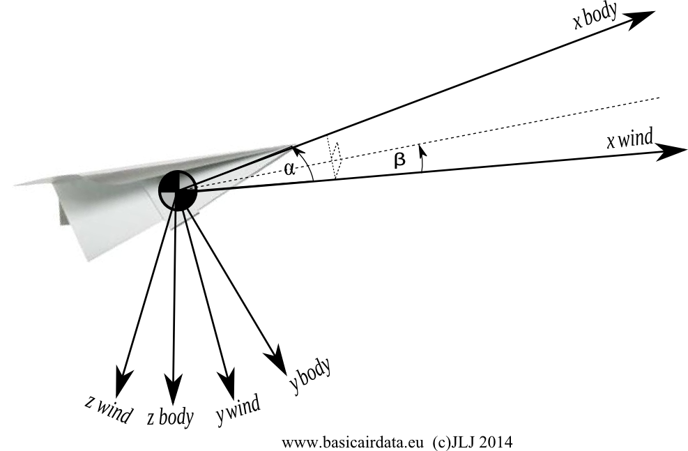
Figure 2 – Body reference frame definition from BAD article

(TP.1) $\begin{equation*} \begin{align} u & = Vcos(\alpha)cos(\beta)\\ v & = Vsin(\beta)\\ w & = Vsin(\alpha)cos(\beta)\\ |V| & = \sqrt{u^2+v^2+w^2} \end{align} \end{equation*}$

If we need to acquire the body velocity for our computations we should convert airspeed to the body frame as per the previous formulas.

Let’s consider a numeric example based on Eq.1. The aircraft is travelling at 100 km/h with $\alpha=10°$ and $\beta=0°$ in a level straight flight path. A planar trajectory is assumed: we’re flying on a vertical plane. In the body frame the velocity expression is $u=98.4 km/h$ and $w=17.5 km/h$

The calculated body velocity should match with the velocity measured by an IMU.

Afterwards, we will investigate the impact of body rotation rates, which create an additional, unwanted velocity component on the tip of the Pitot probe. Since what we are interested in is the center of gravity velocity, the additional velocity should be compensated for. However, this error term does not manifest if the probe tip coincides with the center of gravity, but this would be very unusual.

Let us define the position of the probe tip in the body frame as: $\textbf{p}=\begin{bmatrix} d \\ 0 \\ 0 \end{bmatrix}$

Angular rates in the body frame are: $\boldsymbol{\omega }=\begin{bmatrix} p_b \\ q_b \\ r_b \\ \end{bmatrix}$

These are the roll rate, pitch rate and yaw rate.

The additional speed term at the probe tip is: $\dot{p_b}=\boldsymbol{\omega_b}\times \textbf{p}$

To better understand this error term, let’s assume and examine a planar rotation, $\boldsymbol{\omega_b}=\begin{bmatrix} 0 \\ q_b \\ 0 \\ \end{bmatrix}$ .

We chose a high value for pitch rate $q_b=3 s^{-1}$ that corresponds to about 170 degrees of rotation every second. $\dot{p}=\begin{bmatrix}0\\0\\-dq_b\end{bmatrix}= \boldsymbol{\omega}\times \textbf{p}$ . The body velocity at the probe tip now has a new component along $y_b$ axis with a magnitude of 1.5m/s.

While the body frame makes it easy to deal with vehicle forces and moments, the wind frame provides a better visualization of the impact of body rates on the Pitot probe measurements. However, the question arises: how are body angular rates and wind angular rates related to each other?

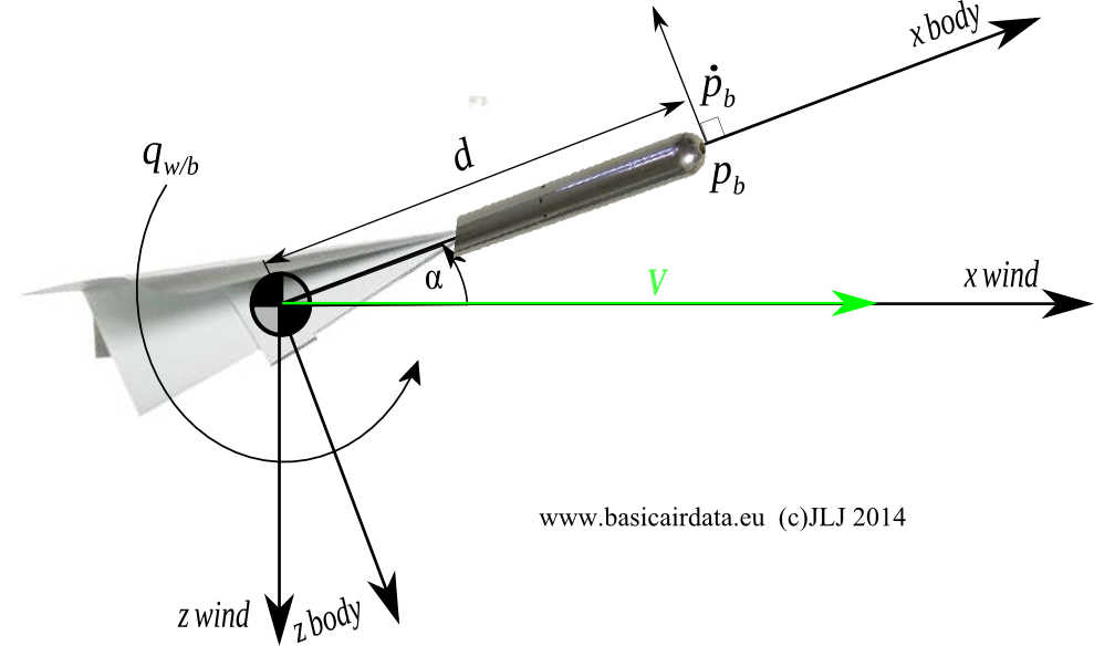
Pitot Correction for Position and Angular Rates figure TP 3

Figure 3 – Problem sketch

Have a look at the Figure 3 that illustrates the problem. The first thing we should do is convert the position vector of the probe tip from body to wind frame.

The coordinates in the wind frame are calculated with the use of a rotation matrix or direction cosine matrix (rotation by angle of attack, then rotation by angle of sideslip)

$R_b^w=\begin{bmatrix}cos(\alpha)cos(\beta) & sin(\beta) & sin(\alpha)cos(\beta) \\-cos(\alpha)sin(\beta) & cos(\beta) & -sin(\alpha)sin(\beta) \\-sin(\alpha) & 0 & cos(\alpha) \end{bmatrix}$

$\textbf{p}_w=R_b^w \textbf{p}_b$

By substitution:

$R_{wb}=\begin{bmatrix} 0.984&0&0.173 \\ 0&1&0 \\-0.173&0&0.984 \end{bmatrix}$

$\textbf{p}_w=\begin{bmatrix}0.984d \\ 0 \\ -0.173d \end{bmatrix}$

Note that the pitot tip distance from cog still the, as expected, equal to d $d_w=\sqrt{0.984^2d^2+0.173^2d^2}=d$ .

The following equation gives the explicit relation between the two angular rates:

$\begin{bmatrix} p_w \\ q_w \\ r_w \end{bmatrix}= R_b^w\begin{bmatrix} p_b-\dot{\beta}sin(\alpha) \\ q_b-\dot{\alpha} \\ r_b+\dot{\beta}cos(\alpha) \end{bmatrix}$

Given $\alpha=10°,\beta=0°,\dot(\alpha),\dot{\beta}=0,p_b=0,q_b=3s^{-1},r_b=0$

$\boldsymbol{\omega}_w=\begin{bmatrix} 0 \\ q_w=q_b \\ r_w \end{bmatrix}= \begin{bmatrix} 0.984&0&0.173 \\0&1&0 \\-0.173&0&0.984 \end{bmatrix} \begin{bmatrix} 0 \\ q_b \\0 \end{bmatrix}$

For this particular case the wind angular rates are identical to the body angular rates. Wind angular rates are correlated also with $\dot{\alpha}$ and $\dot{\beta}$ . Should $\beta$ be non-zero then all the angular rates are coupled with each other.

$\dot{\textbf{p}_w}=\boldsymbol{\omega}_w\times \textbf{p}_w=\begin{bmatrix}-0.259\\0\\-1.47 \end{bmatrix}$

The probe is measuring the true airspeed:

$\textbf{V}=\begin{bmatrix}27.7\\0\\0 \end{bmatrix}=\begin{bmatrix}100 \ km/h\\0\\0 \end{bmatrix}$

plus the speed induced by the rotation.

The resulting airspeed is $\textbf{V}_m=\textbf{V}+\dot{\textbf{p}_w}$ or $\begin{bmatrix}27.4 \\0\\-1.47 \end{bmatrix}$ which yields $|\textbf{V}_m|=27.43 \ m/s$ , hence the error is 1.1%

Neglecting angular rates will introduce an uncertainty in the airspeed measurements and we have evaluated the magnitude of the introduced uncertainty to some degree.

Using the previous formulas, airspeed deviation can be calculated and compensated for, for a given flight condition and for any probe installation position. The overall compensation accuracy should be examined in detail as it’s based on the knowledge of the position of the center of gravity, $\alpha$ , $\beta$ and their derivatives.

In the majority of applications, this compensation is not done due to lack of accurate air data. This analysis can be used to complement the selection of probe installation position.

References

[1]

C. Salter, J. H. Warsap, and D. G. Goodman, “A Discussion of Pitot-Static Tubes and of their Calibration Factors with a Description of Various Versions of a New Design.” Her Majesty’s stationery office, 1965 [Online]. Available: https://naca.central.cranfield.ac.uk/reports/arc/rm/3365.pdf