In this post, I will expose a numerical compensation technique for the acceleration measurements of an airframe, this kind of compensation require the knowledge of airframe angular rates. The measurements are usually available from an Inertial Measurement Unit. Gyroscopes measurements don’t need to be compensated.

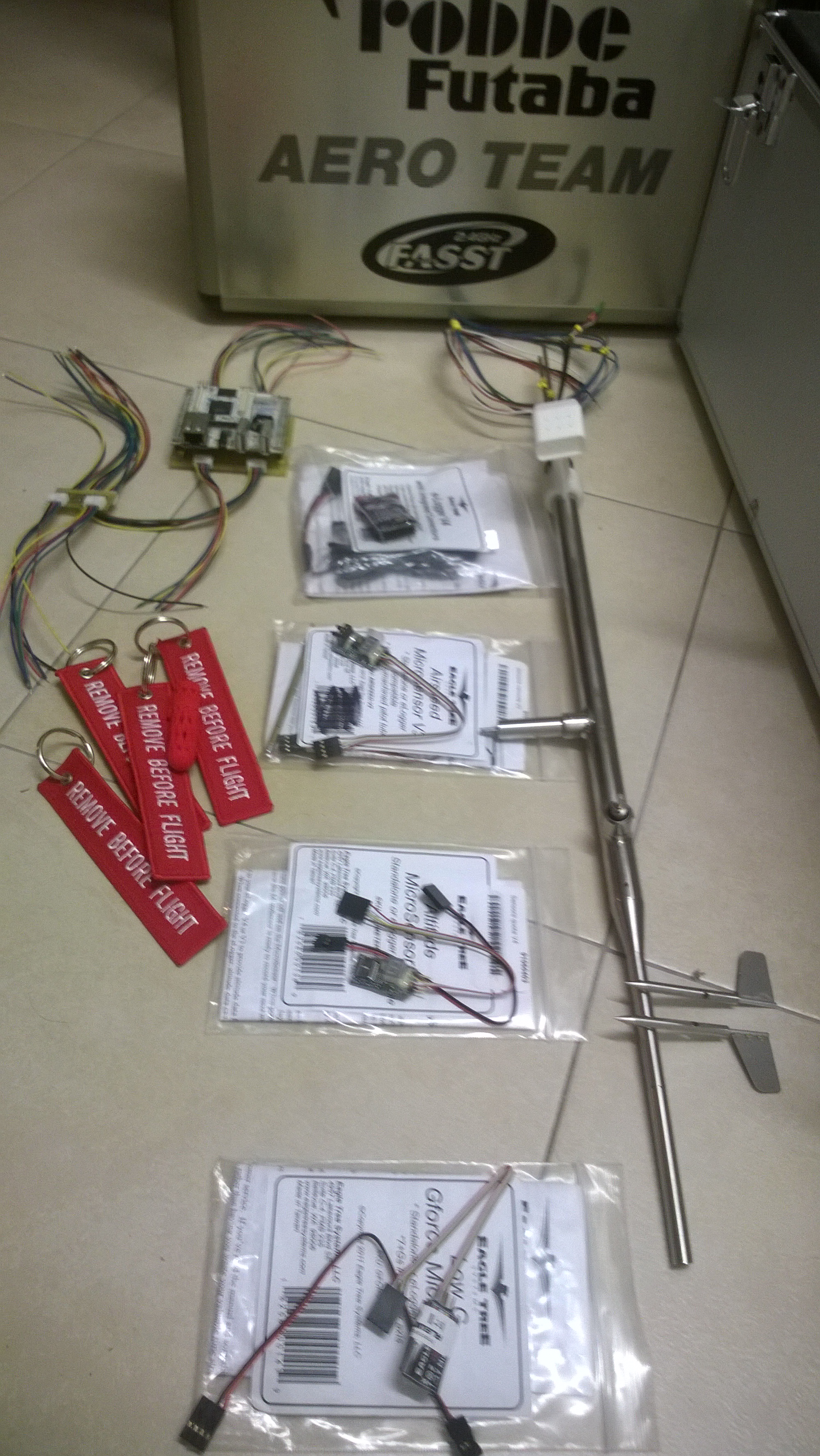
Figure P45.1 – Commercial Eagle tree telemetry system and BasicAirData Air Data Boom
Accelerometers measurements are affected by the position of the IMU respect to the center of gravity. In an ideal layout, the measurements don’t need to be compensated and the accelerometers are placed exactly over the center of gravity C.G., although that will rarely happen.
On many airframes, the center of gravity is located over or near the main spar that fact makes nearly impossible to put the sensor over the C.G.
Even on a middle wing or a low wing plane, this location is often crowded by standard RC equipment. As a general rule the closer is the IMU to the C.G the better; is to bear in mind that compensation for position offset reduces overall accuracy.
The C.G. position should be evaluated in the three dimensions; if the weight, typically affected by fuel consumption or the aerodynamic configuration of the airframe changes during the fly then also the C.G. position should be tracked. This kind of procedures will not be treated here.
The C.G. is the point of rotation of the entire airframe. Let’s use a body-fixed reference system; the origin is set to be coincident with C.G.
On a conventional plane,  coordinate is defined along the airframe from aft to fore,
  is orientated along the right wing and
  points toward the ground. Angular rates respect
  axes are
  . Often
  is called roll rate,
  pitch rate and
  yaw rate. is positive rolling to right, is positive pitching up and is positive yawing right.
The IMU is installed, in the body reference frame, at ![[x_a \quad y_a \quad z_a]^T](http://www.basicairdata.eu/wp-content/ql-cache/quicklatex.com-f22a424f0c2657727f2d0b72fad8f0ca_l3.png "Rendered by QuickLaTeX.com") coordinates. The IMU output is denoted as
coordinates. The IMU output is denoted as ![g[a_xIMU \quad a_yIMU \quad a_zIMU]^T](http://www.basicairdata.eu/wp-content/ql-cache/quicklatex.com-a607a99d7709ca21ccdb5a4523aec6b9_l3.png "Rendered by QuickLaTeX.com")
Refer to the following figure. Let’s examine a planar case. We consider airplane symmetry plane  and set to zero all the angular rates outside this plane; we suppose also small rotation misalignment between body and instrument reference frames [1][2]. The variables for our problem are reduced to
  . If the IMU is placed at a certain distance from C.G. centripetal and tangential acceleration terms affect the measured acceleration.
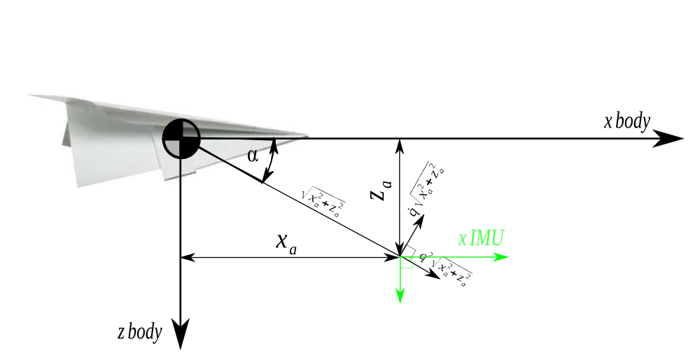
By figure inspection we can write:


It is possible to write the transformation matrix from the body reference frame to
![\[ga_{xC.G.}=ga_{xIMU} + q^2 x_a- \dot{q}z_a\]](http://www.basicairdata.eu/wp-content/ql-cache/quicklatex.com-7b299a12d0206a45f5ba68cd0f0963bb_l3.png "Rendered by QuickLaTeX.com")
That is the explicit relation between measured acceleration and acceleration at C.G.
Suppose we’ve taken an acceleration measurement along x IMU axis of 3g; the IMU position is ![[0.25 \ 0\ 0]^T](http://www.basicairdata.eu/wp-content/ql-cache/quicklatex.com-aedf060dd542d7268caba706cd3ddc7c_l3.png "Rendered by QuickLaTeX.com") ,
,  that is equivalent to a pitch rate of 150° per second.
Calculated acceleration along at C.G.  is 4.7g, we have 36% of offset error in the acceleration measurement. With this simple example is evident the magnitude of the error impact of a casual or undetermined placement of the IMU.
Extending this approach to the three dimensions we can write [1]:
(45.1) 
The last equation confirms our result for the reduced dimensions case previously presented.
Installation position can cause a relevant measurement error, that error is systematic and can be removed from the measurements using equation 45.1.
Further reading
[1] Valdislav Klein and Eugene A. Morelli (2006), Aircraft System Idenification,AIAA
See Chapter 10. Equation 10.12
[2] Gainer, T.G., and Hoffman, S.(1972), Summary of Transformation Equations and Equation of motion Used in Free-Flight and Wind-Tunnel Data Reduction Analysis, NASA
Page 69 Case II, Formula A11-A12-A13
[3] Explicit calculation by ja72 in this link
I quote here in behalf of the reader:
“
Starting from the well known acceleration transformation formula between an arbitrary point _A_ and the center of mass _C_ with  .
.
![\[\vec{a}_C = \vec{a}_A + \dot{\vec{\omega}} \times \vec{c} + \vec{\omega} \times \vec{\omega} \times \vec{c}\]](http://www.basicairdata.eu/wp-content/ql-cache/quicklatex.com-e670f68cb1ca43d1cc7b40eb5b5755ac_l3.png "Rendered by QuickLaTeX.com")
one can you the 3×3 [cross product operator](https://en.wikipedia.org/wiki/Cross_product#Conversion_to_matrix_multiplication) to transform the above into:
![\[\vec{a}_C = \vec{a}_A + \begin{vmatrix} 0 & -\dot{\omega}_z & \dot{\omega}_y \\ \dot{\omega}_z & 0 & -\dot{\omega}_x \\ -\dot{\omega}_y & \dot{\omega}_x & 0 \end{vmatrix} \vec{c} + \begin{vmatrix} 0 & -\omega_z & \omega_y \\ \omega_z & 0 & -\omega_x \\ -\omega_y & \omega_x & 0 \end{vmatrix} \begin{vmatrix} 0 & -\omega_z & \omega_y \\ \omega_z & 0 & -\omega_x \\ -\omega_y & \omega_x & 0 \end{vmatrix} \vec{c}\]](http://www.basicairdata.eu/wp-content/ql-cache/quicklatex.com-c8547fb0823d13c0a4f8722936634602_l3.png "Rendered by QuickLaTeX.com")
or in the form seen the linked post:
![\[\vec{a}_C = \vec{a}_A + \begin{vmatrix}-\omega_y^2-\omega_z^2 & \omega_x \omega_y - \dot{\omega}_z & \omega_x \omega_z + \dot{\omega}_y \\ \omega_x \omega_y + \dot{\omega}_z & -\omega_x^2-\omega_z^2 & \omega_y \omega_z + \dot{\omega}_x \\ \omega_x \omega_z - \dot{\omega}_y & \omega_y \omega_z + \dot{\omega}_x & -\omega_x^2 - \omega_y^2 \end{vmatrix} \vec{c}\]](http://www.basicairdata.eu/wp-content/ql-cache/quicklatex.com-55394f908261b3155d602d53a7a80212_l3.png "Rendered by QuickLaTeX.com")