Check this article, 8mm BAD probe was tested within a wind tunnel
Test and calibration represents the difference between obtaining meaningful data or not. Calibration is a preliminary phase, non necessary involving any flight activity as wind tunnel activity, that provide a systematic procedure to determinate the operating parameters for the pitot. Test is refereed to the routine procedures that must me carried out to be sure, to some degree of confidence, that our instrument is operating good. Here it will outline some basic procedure, that come mostly after the DIY approach. At the end we will add uncertainty information to our measure.
Calibration
Our objective here is to verify the degree of accuracy of our readings, experimental data is the most valuable source of information. In reference[1] there are some description of practical means to calibrate full size airplanes instruments, an alternative inflight approach is used in [2]. The method described in ref[2] is of course the most appealing, I’ve using it for a while but for sake of simplicity I present one most basic procedure. The flight plan consist on a series of runway flybies, ideally at the same height and speed; if some sort of fly aiding, i.e .altitude control, is available use it. As no wind compensation will be used try to fly in a calm day, best conditions usually are in the early morning or in the late afternoon. The RC airfield I use is often covered by fog, so ideal conditions are at my reach; sometimes in the morning there is no detectable wind but the model is anyway flyable also if a thin fog is present.
Remembering the considerations on calibration factor of pitot page, it’s safe to reduce our calibration to one point, with this degree of approximation a speed variation of some m/s will not change the calibration parameter fact that simplifies our data collection task.
Measured variables should be at least:
- Ambient Temperature, at ground station;
- Ambient Pressure, at ground station;
- Pitot differential pressure;
- GPS speed;
- Time stamp for each measure;
Will increase accuracy also to know
- Ambient Relative Humidity;
To aid datum selection we may need information about our position:
- GPS position, if we flight near the ground station at low altitude ground measured pressure, temperature and humidity will be more likely those of the air surrounding our aircraft.
Regarding altitude with a medium size aircraft ten meters should work, choice an altitude where you can see clearly the model and fly it confident. Flying too high will introduce errors due to wind and generally air density variations. Ever consider safety indication of your flying field.
Use sensors with a know uncertainty and note it within the sensor logs, soon or later you may need that info. Every accessory sensor that you intend to use for the calibration should be calibrated himself.
Indeed only one point calibration is sufficient to calibration however for validation purposes it’s wise to collect at last some data serie at a substantial different speed (let’s say at last 10 m/s different), if the pitot is manufactured and installed correctly the calibration factor calculated with the two data sets will be the same; cross validation procedure should be applied.
Recall the basic dynamic pressure formula from pitot page:
(1) 
From all the available experimental data use mainly parts of your log where you find:
- Straight fly segments
- Limited speed variations
- Limited altitude variations
- Aircraft proximity to base station, to use the best temperature and pressure readings.
Aided by eventually GPS data you can easy isolate good samples, once done proceed to sort data by crescent speed to have an immediate feedback on speed dispersion. By experience the data collected by man piloted RC model runway flyby are good to use.
For every sample compute a csample value with the following formula:
(2) 
Note that if normal probability function is choose to fit the distribution of speed, deltap and (\rho\) sample probability then the single csample should not be normal distribuited but the average[3] of csample should be normally distributed no matter what probability function have the single sample.
Searched calibration factor c value is the mean of all csamples, also the standard deviation can be calculated from raw data, if the probability distribution is proof to be normal then our fast analysis is done and consistent. Check this example spreadsheet.
Look at the tab labeled one on the spreadsheet, here we visualize probability distribution and compare it with a normal distrubution by mean of a Quantile vs Quantile graph.
This is a preliminary steep to quickly verify is our data seem good, a good pratice is to calculate the squared error sum, as per the example spreadsheet; with SES you can pretty fast verify different data sets.
Now focus on the tab labeled two;
We know that once we dispose of a large set of data it’s possible to calculate the average and the standard deviation, this two values are the final measure value and the accuracy.
In the spreadsheet, using Nist[4] Error propagation formula, the accuracy is calculated a priori. In some way this value is the better result that we can expect to attain.
In the example the density is assumed constant during all the measures. This is a simplication, typically a measure of (\rho\) should be made at the same time of the deltap and speed measures.
Check also the spreadsheet for the assumed values of every measure uncertainty. Please note that in the spreadsheet it’s assumed that air is dry for density calculation, clearly that is not true and lead to an additional uncertainty, to increase precison please refer to the calculation procedure for air density. Following the link you get also a useful software to carry out uncertainty calculations. The density calculated with this method is used to compensate for buoancy in laboratory measurements.
Routine Test
As often as you can it is necessary to check your pitot basic functionality. Common problems are sensor aging with correlated reading drift, pressure line clogging and condensate related problems. When you calibrate you sensor for the first time of course you made an offset adjustment so at no speed the reading from the sensor is zero, if some time passes the sensor naturally drift; checking at ground the reading can detect a deviation from zero. When the reading is moved only of some percent fraction you can compensate it with the software and go ahead with the flight, follow this link for an example software.
Another test is the following, put half scale pressure on the total pressure port and read the sensor output, if the reading is 1/4 FS IAS your pitot sensor and electronics is performing correctly.
To prevent clogging always put a protection over the pitot tip and the static port.
On a regular basis drain the condensate from the pressure lines, refer to this page for a basic connection scheme with drain lines.
Uncertainty of measurement
Pitot measurement system have been modeled only at a hardware level. Every uncertainty derives from the measurement procedure, manufacturing and aerodynamics. Let’s defines as primary instrument part everything that compose the physical device that interact with the air and as secondary the pressure sensor and the auxiliary electronics. With this new definitions we can say that until now only the primary have been treated to some degree.
The plan is to obtain an uncertainty for the primary instrument and account for secondary uncertainty in an independent manner. Divide et impera approach eases the engineering and operational burden. From the previous paragraph it is defined the calibration factor:
c with u(c) uncertainty equal to 0.005, that represent the whole uncertainty from primary.
Dealing with the secondary
Regarding secondary it’s needed information about differential pressure and air density uncertainty, it’s assumed that pneumatic connection is well designed so don’t impact on performances. Best method to determine uncertainty is the experimental one, a numerical estimation is anyway useful for a priori system performance evaluation and design.
Considering a typical application where the instrument gives IAS and TAS main sources of uncertainty are:
- Differential pressure sensor;
- Signal conditioning, Analog to digital converter;
- Air density;
- Calculation rounding;
To obtain a robust preliminary estimation it’s wisely to operate in a worst case scenario, some times this assumption is so brutal that dramatically overestimate measure uncertainty; Uncertainty value will be function of current speed, air temperature and pressure so for a most reliable result every accuracy term should be calculated with the current operating values. If a digital sensor, with a non ratiometric output, is used the main thing that we should check is the temperature compensation range, the wider the better. Use of analog sensors introduce supplementary issues related with power supply stability and temperature of sensor itself and of the signal conditioning circuit; in this case uncertainty analysis should be carried out carefully and is out of the scope for this example application. Let’s proceed assuming that a digital sensor is used.
Producers of low cost differential pressure sensors usually give accuracy information in term of % over the range, let’s use 1% for example purposes.
Hence u(q) is 1% of range.
Regarding air density we should evaluate or retrieve:
- Uncertainty of density equation
- Impact of other measured variables on the density calculation
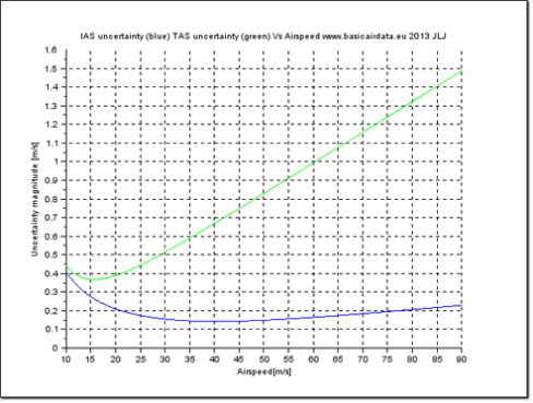
Figure 1 – Comparison between IAS (Blue) and TAS (Green) uncertainty value versus airspeed
If we calculate density using pressure and temperature measurements it’s advisable to account for error propagation.
This approach have been used in this example scilab (missed link) file, refer also to this documentation for density calculation.
Calculation rounding seems trivial in year 2013 but is not indeed, if we deal with variables or parameters that have a wide range i.e. 10e3 to 10e-10 it’s must be assured that we dispose of suitable data types, cheap microcontrollers may have only 8 bits data operators and operations.
![\[IAS=\sqrt{\frac {2qc}{\rho_{s}}}\]](https://www.basicairdata.eu/wp-content/ql-cache/quicklatex.com-6f59d3e6c109b697baddc52a967e19fd_l3.png "Rendered by QuickLaTeX.com")
with density fixed to standard value of  given
given  , in the spreadsheet the uncertainty is calculated using propagation formula [4].
Recalling the TAS formula:
![\[TAS=CAS\sqrt{\frac{\rho_{s}}{\rho_{a}}}\]](https://www.basicairdata.eu/wp-content/ql-cache/quicklatex.com-61b3b6234ff6ee112736c8548c936e90_l3.png "Rendered by QuickLaTeX.com")
In this case the current density should be know, usually it is calculated using a formula that use temperature and pressure, humidity is neglected. This approximation lead an important reading error, nevertheless humidity in flight measurement is not practical; to reduce the error can be usefull to considerate RH fixed at 50%. Here below I report a figure that shown uncertainty value for IAS and TAS in reference to the speed, details on parameters and figure are at disposal executing the example scilab file.
As expected IAS uncertainty is anytime below TAS uncertainty, the former uncertainty should be higher because it consider also density error contribution.
Now we dispose of a minimal scheme and procedure to accuracy estimation so it’ s possible to select the correct hardware in function of our goal uncertainty.